|
Dr. N.K.Dashora Guest Faculty Rajeev Gandhi Tribal University Udaipur |
Sunil Kumar Research scholar Pacific University Udaipur Email: narandrad@gmail.com |
Recent upheaval in the crude oil price in international market has created renewed interest in the data analysis. But even before this, the energy reports generated internationally have squarely yelled about growing crude oil consumption in India and China. India’s share of global demand rises to 8% in 2035, accounting for the second largest share of the BRIC countries with China at 26%, Russia 5%, and Brazil 3%.The object of this paper is to find out whether the price changes and income changes have the same impact on the elasticity of consumption as shown in the theory of elasticity of demand. The yearly data used are from 1985 to 2013.The log value of consumption, income and the adjusted inflation price gives the best results. The coefficient values have been estimated for price and income elasticity.
Keywords: Crude Oil, Consumption, India.
While the crude oil consumption has always been a matter of concern internationally, it has direct implication for self sufficiency, overall prices and for the balance of payments. Recent upheaval in the crude oil price in international market has created renewed interest in the data analysis. But even before this, the energy reports generated internationally have squarely yelled about growing crude oil consumption in India and China. The rising population and higher growth trajectory has put this demand on international map. India was the fourth-largest consumer of crude oil and petroleum products in the world in 2013, after the United States, China, and Japan. The country depends heavily on imported crude oil, mostly from the Middle East.
The three startling remarks about projection of India ‘s demand for future in coming twenty years are as following :
(i) India’s share of global demand rises to 8% in 2035, accounting for the second largest share of the BRIC countries with China at 26%, Russia 5%, and Brazil 3%.
(ii) India’s demand growth of 128% outpaces each of the BRIC countries as Russia (+14%), China (+60%) and Brazil (+72%) all expand more slowly. India’s growth is almost double the non-OECD aggregate of 63%.
(iii) India’s energy production as a share of consumption declines from 59% today to 56% by 2035; imports rise by 143%. (BP Energy Outlook 2035).
Similar concerns have been echoed by International Energy Association and US energy Information and other global reports.
The object of this paper is to find out the association between growth in income and the energy price .The research question is to estimate the validity of the statement that price elasticity of crude oil consumption is negative and the income elasticity is positive.
H0 1. The price elasticity of demand is negative and significant
H1. 1. The price elasticity of demand is positive and significant
H o. 2 The income elasticity of demand is positive and significant
H 1 2. The price elasticity of demand is negative and significant
Several studies on India use the ordinary least square (OLS) method (Goldar and
Mukhopadhyay 1990; Rao & Parikh 1996; Parikh et al., 2007), but most variables involved are actually non-stationary. Other studies that used co-integration
techniques focused on petroleum derivatives (Ramanathan 1999; Ghosh 2010; Chemin
2012) or on demand for imported oil only (Ghosh 2009). Thus, none of these studies
estimates and forecasts the total crude oil demand for India. The studies that estimate
imported crude oil demand (Ghosh 2009) used, with data until 2005–06. Pradeep Agrawal (2012) empirically estimated demand relations for crude oil, diesel, and petrol for India using the ARDL co-integration procedure and data from 1970 to 2011. These estimations show the income elasticity of about 1 for crude oil and diesel and 1.39 for petrol. The price elasticity of the petroleum products was found to be negative and statistically significant in all the models. The values of price elasticity estimates were found to be -0.41, -0.56 and -0.85 for crude oil, diesel, and petrol respectively, While the absolute value is less than one that inelastic the sign shows the inverse relationship between price rise and demand.
Data
For uniformity the data used are from Energy Statistics 2014 and its prior editions. In case of adjusted inflation price of crude oil the data are from Index Mundi. It may be acknowledged that international crude oil price data do not fully reflect the price behavior for the simple reason that several adjustments are made in fixing the price.
Summary Statistics, using the observations 1985 – 2013
| Variable | Mean | Median | Minimum | Maximum |
| Reserves | 5.36413 | 5.60635 | 3.50000 | 7.99710 |
| Production | 665.568 | 661.420 | 534.000 | 782.340 |
| consumption | 2064.53 | 2031.25 | 894.900 | 3509.00 |
| Nominalprice | 36.6762 | 23.0000 | 11.9100 | 91.4800 |
| InflationAdjusyedPrice | 47.2155 | 35.5500 | 17.2600 | 100.010 |
| PCINNP | 22177.7 | 20079.0 | 12095.0 | 39904.0 |
| Variable | Std. Dev. | C.V. | Skewness | Ex. kurtosis |
| Reserves | 1.01209 | 0.188677 | 0.398414 | 0.527339 |
| Production | 58.4482 | 0.0878170 | 0.115065 | 0.180980 |
| consumption | 830.729 | 0.402382 | 0.180061 | -1.25816 |
| Nominalprice($) | 26.5740 | 0.724557 | 1.05374 | -0.405856 |
| InflationAdjusyedPrice($) | 24.2479 | 0.513558 | 0.882616 | -0.570873 |
| PCINNP | 8838.14 | 0.398516 | 0.722700 | -0.771556 |
The summary statistics indicate that production and consumption have normal distribution but Reserves and prices and per capita income are skewed. Also there is Excess Kurtosis (> 3 ) in each of these variables. We examine the crude oil consumption as dependent variable and per capita income and nominal price as repressors. Both the sign are statistically significant.
Model 1: OLS, using observations 1985-2013 (T = 29)
Dependent variable: consumption
| Coefficient | Std. Error | t-ratio | p-value | ||
| const | -232.105 | 115.004 | -2.0182 | 0.05400 | * |
| PCINNP | 0.121084 | 0.00942236 | 12.8507 | <0.00001 | *** |
| Nominal_price | -10.5987 | 3.13375 | -3.3821 | 0.00229 | *** |
| Mean dependent var | 2064.527 | S.D. dependent var | 830.7289 | |
| Sum squared resid | 700213.8 | S.E. of regression | 164.1076 | |
| R-squared | 0.963763 | Adjusted R-squared | 0.960975 | |
| F(2, 26) | 345.7479 | P-value(F) | 1.86e-19 | |
| Log-likelihood | -187.4810 | Akaike criterion | 380.9619 | |
| Schwarz criterion | 385.0638 | Hannan-Quinn | 382.2466 | |
| rho | 0.660907 | Durbin-Watson | 0.681402 |
.gif)
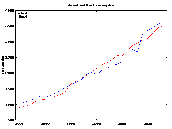
From the model one it is obvious that the per capita income has positive and price has negative sign.R-Square is sufficiently high.Though DW statistic is low.
Model 2: OLS, using observations 1985-2013 (T = 29)
Dependent variable: consumption
| Coefficient | Std. Error | t-ratio | p-value | ||
| const | 4.27255 | 82.1937 | 0.0520 | 0.95894 | |
| PCINNP | 0.110539 | 0.00627453 | 17.6171 | <0.00001 | *** |
| Inflation Adjusted Price | −8.28634 | 2.28701 | −3.6232 | 0.00124 | *** |
| Mean dependent var | 2064.527 | S.D. dependent var | 830.7289 | |
| Sum squared residual | 669989.9 | S.E. of regression | 160.5268 | |
| R-squared | 0.965327 | Adjusted R-squared | 0.962660 | |
| F(2, 26) | 361.9313 | P-value(F) | 1.05e-19 | |
| Log-likelihood | −186.8412 | Akaike criterion | 379.6824 | |
| Schwarz criterion | 383.7843 | Hannan-Quinn | 380.9670 | |
| rho | 0.695536 | Durbin-Watson | 0.617639 |

Model 2 denotes inflation adjusted price. The model is slightly improved as far as Akaike and other criterion are concerned. However the predictive ability is hardly improved in this model as compared to model 1 above.
Model 3: OLS, using observations 1985-2013 (T = 29)
Dependent variable: l_consumption
| Coefficient | Std. Error | t-ratio | p-value | ||
| const | −6.02301 | 0.692683 | −8.6952 | <0.00001 | *** |
| l_PCINNP | 1.44244 | 0.0841815 | 17.1348 | <0.00001 | *** |
| l_Nominalprice | −0.224841 | 0.0492504 | −4.5653 | 0.00011 | *** |
| Mean dependent var | 7.546872 | S.D. dependent var | 0.432760 | |
| Sum squared resid | 0.158264 | S.E. of regression | 0.078020 | |
| R-squared | 0.969819 | Adjusted R-squared | 0.967498 | |
| F(2, 26) | 417.7375 | P-value(F) | 1.72e-20 | |
| Log-likelihood | 34.40719 | Akaike criterion | −62.81438 | |
| Schwarz criterion | −58.71250 | Hannan-Quinn | −61.52972 | |
| rho | 0.634979 | Durbin-Watson | 0.741173 |

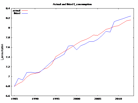
Model 3 is Double log model, with the same set of variables. From this the price elasticity and the income elasticity of consumption can be directly read out. The Akaike and other criterion have improved greatly. The DW statistic has slightly improved.
Model 4: OLS, using observations 1985-2013 (T = 29)
Dependent variable: l_consumption
| Coefficient | Std. Error | t-ratio | p-value | ||
| const | −4.60602 | 0.408795 | −11.2673 | <0.00001 | *** |
| l_PCINNP | 1.30804 | 0.0508049 | 25.7463 | <0.00001 | *** |
| l_InflationAdjusyedPrice | −0.225224 | 0.0401918 | −5.6037 | <0.00001 | *** |
| Mean dependent var | 7.546872 | S.D. dependent var | 0.432760 | |
| Sum squared resid | 0.129148 | S.E. of regression | 0.070479 | |
| R-squared | 0.975372 | Adjusted R-squared | 0.973477 | |
| F(2, 26) | 514.8442 | P-value(F) | 1.23e-21 | |
| Log-likelihood | 37.35508 | Akaike criterion | −68.71015 | |
| Schwarz criterion | −64.60826 | Hannan-Quinn | −67.42549 | |
| rho | 0.574011 | Durbin-Watson | 0.852549 |

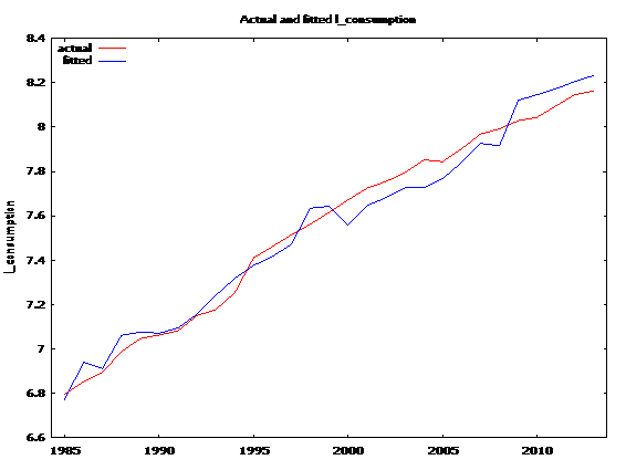
In model 4 the variable choosen are the same as in model 2 that is inflationary adjustement price. There is again an improvement in the model. This model stands the best as far as predictive ability is concerned. The DW statistic too has improved.While the sign and value of the price change remain almost the same , ther is decline in income elasticity of demand . This might be the result of common trend in the inflation and income variables.Since these are yearly data much conversion of income and price takes place within a year therefore lagged data have not been used .
BP Energy Outlook 2035, http://www.bp.com/en/global/corporate/about-bp/energy-economics/energy-outlook/country Insight India
Chemin, Elodie Sentenac (2012), “Is the price effect of fuel consumption symmetric? Some evidence from an empirical study”, Energy Policy, 41, 59-65.
Ghosh, Sajal (2006), “Future demand of petroleum products in India”, Energy Policy, 34, 2032-2037.
Ghosh, Sajal (2009), “Import demand of crude oil and economic growth: Evidence from India”, Energy Policy, 37, 699-702.
Ghosh, Sajal (2010), “High speed diesel consumption and economic growth in India”, Energy, 35, 1794-1798.
Goldar, Bishwanath. And Mukhopadhyay, Hiranya., (1990), “India’s Petroleum Imports: An Econometric Analysis”, Economic Political Weekly, 25 (42/43), 2373-2377
Parikh, Jyoti., Purohit, Pallav. And Maitra, Pallavi., (2007), “Demand projections of petroleum products and natural gas in India”, Energy, 32, 1827-1837.
Pradeep Agrawal (2012) Empirical Estimations and Projections for the Futurewww IEG Working Paper No. 319 , 2012, Institute of Economic Growth Dehli : , http://www.iegindia.org.
Ramanathan, R. (1999), “Short- and long-run elasticities of gasoline demand in India: An empirical analysis using cointegration techniques”, Energy Economics, 21, 321-330.
Rao, Raghavendra D and Parikh, Jyoti K. (1996), “Forecast and analysis of demand for petroleum products in India”, Energy policy, 24(6), 583-592.