Abstract

In this paper, we have analysed a deterministic inventory model for deteriorating items with time-dependent quadratic demand and holding cost is time-dependent. An Exponential distribution is used to represent the distribution of time to deterioration . In the model considered here, shortages are allowed and partially backlogged. The backlogging rate is assumed to be dependent on the length of waiting for the next replenishment. The longer the waiting time is, the smaller the backlogging rate would be. The model is solved analytically to obtain the optimal solution of the problem. The derived model is illustrated by a numerical example and its sensitivity analysis is carried out.

Keywords

Deteriorating items,Exponential distribution ,Inventory, Partial backlogging, Quadratic demand, Shortages,Time-varying holding cost.

Introduction

Inventory system is one of the main streams of the Operation Research which is essential in business enterprises and industries.Inventory may be considered as an accumulation of a product that would be used to satisfy future demands for that product. It needs scientific way of exercising inventory model.

An optimal replenishment policy is dependent on ordering cost, inventory carrying cost and shortage cost. An important problem confronting a supply manager in any modern organization is the control and maintenance of inventories of deteriorating items. Fortunately, the rate of deterioration is too small for items like steel, toys, glassware, hardware, etc. There is little requirement for considering deterioration in the determination of economic lot size.

Inventory of deteriorating items first studied by Whitin (1957), he considered the deterioration of fashion goods at the end of prescribed storage period. Ghare and Schrader (1963) extended the classical EOQ formula to include exponential decay, wherein a constant fraction of on hand inventory is assumed to be lost due to deterioration.Covert and Philip (1973) and Shah and Jaiswal (1977) carried out an extension to the above model by considering deterioration of Weibull and general distributions respectively. Dave and Patel (1981)first developedan inventory model for deteriorating items with time proportional demand, instantaneous replenishment and no shortagesallowed. Many researchers such as Park (1982)and Hollier and Mak (1983) also considered constant backlogging rates in their inventory models. Nahmias (1978) gave a review on perishable inventory theory. Rafaat (1991) described survey of literature on continuously deteriorating inventory model. He focused to present an up-to-date and complete review of the literature for the continuously deteriorating mathematical inventory models.

All researchers assume that during shortage period all demand either backlogged or lost. In reality, it is observed that some customers are willing to wait for the next replenishment. Abad (1996) considered this phenomenon in his model, optimal pricing and lot sizing under conditions of perishable and partial backordering. He assume that the backlogging rate depends upon the waiting time for the next replenishment. But he does not include the stock out cost (back order cost and lost sale cost).

Goyal and Giri (2001) gave recent trends of modeling in deteriorating inventory. Ouyang, Wu and Cheng (2005) developed an inventory model for deteriorating items with exponential declining demand and partial backlogging. Dye and Ouyang (2007) found an optimal selling price and lot size with a varying rate of deterioration and exponential partial backlogging. They assume that a fraction of customers who backlog their orders increases exponentially as the waiting time for the next replenishment decreases. Singh and Singh (2007) presented an EOQ inventory model with Weibull distribution deterioration, Ramp type demand and Partial Backlogging. NitaShah and Kunal Shukla (2009) developed a deteriorating inventory model for waiting time partial backlogging when demand is constant and deterioration rate is constant. Singh,T.J., Singh, S.R. and Dutt, R. (2009) extended an EOQ model for perishable items with power demand and partial backlogging.Skouri, Konstantaras, Papachristos and Ganas (2009) developed an Inventory models with ramp type demand rate, partial backlogging and Weibell's deterioration rate.

An exponentially time-varying demand also seems to be unrealistic because an exponential rate of change is very high and it is doubtful whether the market demand of any product may undergo such a high rate of change as exponential.

In reality, the demand and holding cost for physical goods may be time dependent. Time also plays and important role in the inventory system. So, in this paper we consider that demand and holding cost are time dependent.

Recently, Mishra and Singh (2011) developed a deteriorating inventory model with partial backlogging when demand and deterioration rate is constant. Vinodkumar Mishra (2013) developed an inventory model of instantaneous deteriorating items with controllable deterioration rate for time dependent demand and holding cost.

J. Jagadeeswari and P. K. Chenniappan (2014) developed an order level inventory model for deteriorating items with time – quadratic demand and partial backlogging. Sarala Pareek and Garima Sharma (2014) developed an inventory model with Weibull distribution deteriorating item with exponential declining demand and partial backlogging. R. Amutha and Dr. E. Chandrasekaran developed an inventory model for deteriorating items with time – varying demand and partial backlogging.Kirtan Parmar and U. B. Gothi(2014) developed a deterministic inventory model for deteriorating items where time to deterioration has Exponential distribution and with time-dependent quadratic demand. In this model, shortages are not allowed and holding cost is time-dependent. Also, U. B. Gothiand Kirtan Parmar(2015) have extended above deterministic inventory model by taking two parameter Weibull distribution to represent the distribution of time to deterioration and shortages are allowed and partially backlogged. Kirtan Parmar and U. B. Gothi (2015) developed an economic production model for deteriorating items using three parameter Weibull distribution with constant production rate and time varying holding cost.

In this paper, we have analysed an inventory system order level lot size model for deteriorating items under quadratic demand and time dependent IHC.

Notations

The mathematical model is developed using the following notations:

01. Q(t) : The instantaneous state of the inventory level at any time t. (0 ≤ t ≤ T)

02. R(t) : Quadratic demand rate.

03. A : Ordering cost per order.

04. C_h : Inventory holding cost per unit per unit time.

05. C_d : Deterioration cost per unit per unit time.

06. Cs : Shortage cost due to lost sales per unit.

07. Q : Order quantity in one cycle.

08. p_c : Purchase cost per unit.

09. l : Opportunity cost due to lost sales per unit.

10. t₁ : The time at which the inventory level reaches zero (decision variable)

11. T : Length of cycle time (decision variable).

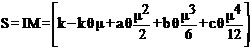
12. IM : The maximum inventory level during [0, T].

13. IB : The maximum inventory level during shortage period.

14. TC(t₁,T) : Total cost per unit time.

Assumptions

The model is derived under the following assumptions.

1. The inventory system deals with single item.

2. The annual demand rate is a function of time and it is R(t) = a+bt+ct² (a, b, c > 0)

3. Holding cost is linear function of time and it is C_h = h + rt (h, r > 0)

4. The lead time is zero.

5. Time horizon is finite.

6. No repair or replacement of the deteriorated items takes place during a given cycle.

7. Total inventory cost is a real, continuous function which is convex to the origin.

8. Shortages are allowed and partially backlogged.

During stock out period, the backlogging rate is variable and is dependent on the length of the waiting time for the next replenishment. The backlogging rate is assumed to be where the backlogging parameter δ (0< δ<1) is a positive constant and (T – t) is waiting time (t₁ ≤ t ≤ T).

Mathematical Model And Analysis

Here, the replenishment policy of a deteriorating item with partial backlogging is considered. The objective of the inventory problem is to determine the optimal order quantity and the length of ordering cycle so as to keep the total relevant cost as low as possible. The behavior of inventory system at any time is shown in Figure 1.

Replenishment is made at time t = 0 and the inventory level is at its maximum level S. During the period [0, μ] the inventory level is decreasing and at time t₁ the inventory reaches zero level, where theshortages starts and in the period [t₁, T] some demands are backlogged.

The pictorial representation is shown in the Figure 1.

As described above, the inventory level decreases owing to demand rate as well as deterioration during inventory interval [0, t₁]. Hence, the differential equation representing the inventory status is given by

(1)

(2)

During the shortage interval [t₁,T], the demand at time t is partly backlogged at the fraction . Thus, the differential equation governing the amount of demand backlogged is as below.

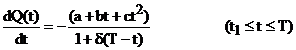(3)

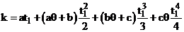
The boundary conditions are Q(0) = S, Q(t₁) = 0 and Q(T) = 0. (4)

Using the boundary condition Q(0) = S the solution of equation (1) is

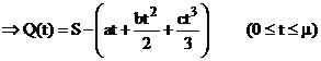(5)

Similarly, the solution of equation (2) is given by

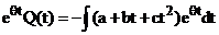
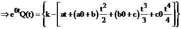(neglecting higher powers of θ)

(where which is obtained using Q(t₁) = 0)

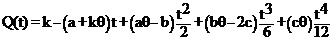(μ ≤ t ≤ t₁) (6)

In equations (5) and (6) values of Q(t) should coincide at t = μ, which implies that

(7)

Solution of equation (3) is given by

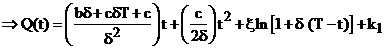(8)

(where k₁ is the constant of integration and )

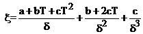With boundary condition Q(t₁) = 0, we get

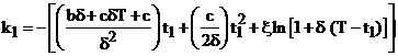(9)

Therefore, from (8) and (9)

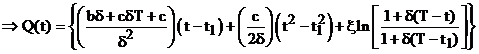(t₁ ≤ t ≤ T) (10)

The total cost comprises of following costs

1) The ordering cost

OC = A (11)

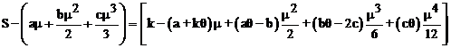
2) The deterioration cost during the period [μ, t₁]

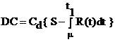
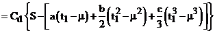(12)

3) The inventory holding cost during the period [0, t₁]

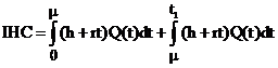
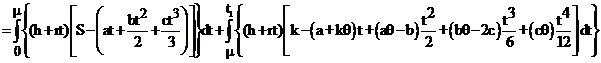
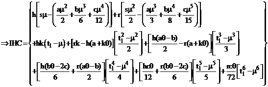(13)

4) The shortage cost per cycle

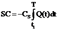
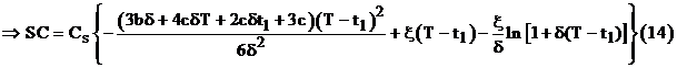
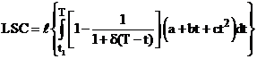
5) Lost sales cost per cycle

The maximum backordered inventory is obtained at t = T and it is denoted by IB. Then from equation (10),

IB = – Q(T)

(16)

Thus, the order size during total interval [0, T] is given by

6) Purchase cost per cycle

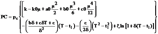(17)

Hence the total cost per unit time is given by

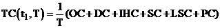
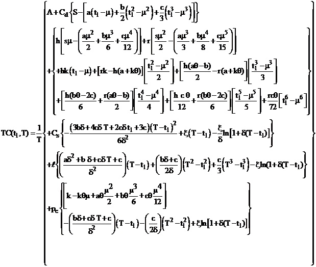(18)

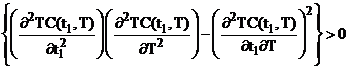
Our objective is to determine optimum value of t₁ and T so that TC(t₁,T) is minimum. The values of t₁ and T, for which the total cost TC(t₁,T) is minimum, is the solution of equations 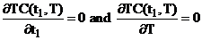satisfying the condition

The optimal solution of the equations (18) can be obtained by using appropriate software. This has been illustrated by the following numerical example.

Numerical Example

We consider the following parametric values for A = 300, a = 10, b = 8, c = 5, h = 1, r = 0.5,

μ = 1, θ = 0.02, δ = 0.03, C_d = 5, p_c = 15, ℓ = 10, Cs = 2.

We obtain the optimal value of t₁ = 0.9483421102 units, T = 1.577867692 units and optimal total cost (TC) = 558.4065267.

Sensitivity Analysis

Sensitivity analysis depicts the extent to which the optimal solution of the model is affected by the changes or errors in its input parameter values. In this section, we study the sensitivity of the total cost per time unit TC(t₁,T) with respect to the changes in the values of the parameters A, a, b, c, h, r, δ, θ, μ, Cd, Cs, ℓ , pc.

The sensitivity analysis is performed by considering 10% and 20% increase or decrease in each one of the above parameters keeping all other parameters the same. The results are presented in Table – 1.

Table – 1 :Partial Sensitivity Analysis

Graphical Representation

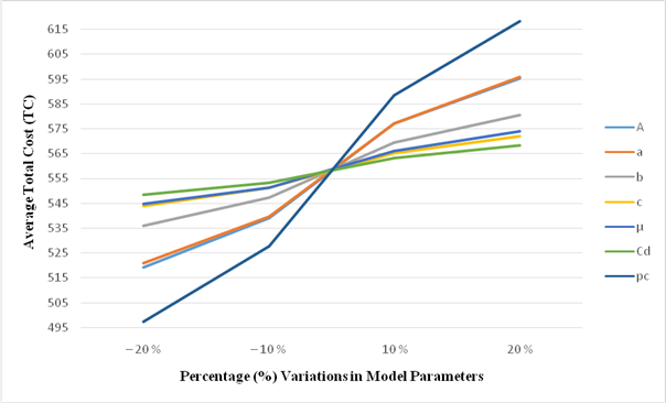
Figure – 2

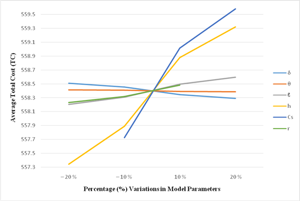
Figure –3

Conclusions

Ø It is observed from Figure – 2 that total cost per unit time (TC) is highly sensitive to changes in the value of p_c, moderately sensitive to changes in the values of A, a and less sensitive to changes in the values of b, c, μ, C_d.

Ø It is observed from Figure – 3 that total cost per unit time (TC) is highly sensitive to changes in the values of h and Cs, moderately sensitive to changes in the values of ℓ, r, δ and less sensitive to change in the values of θ.

References

1. Abad, P. L., (1996) , “Optimal pricing and lot-sizing under conditions of perishability and partial backordering. Management Science, 42, 1093 – 1104.

2. Chang H.J., Dye C.Y., (1999) , “An EOQ Model for deteriorating items with time - varying demand and partial backlogging”, Journal of Operational Research Society,50, pp. 1176 – 1182.

3. Covert R.P., and Philip G.C. (1973) , “An EOQ model with Weibull distribution deterioration”, American Institute of Industrial Engineers Transaction, Vol. 5, pp. 323 – 326.

4. Dave U, and Patel L.K. (1981), “(T, Si) policy inventory model for deteriorating items with time proportion demand”, Journal of Operational Research Society, 32, pp.137 – 142.

5. Dye C. Y., Ouyang LY, Hsieh TP (2007) “Deterministic inventory model for deteriorating items with capacity constraint and time-proportional backlogging rate.” European Journal of Operational Research, 178(3), pp. 789-807.

6. Ghare, P. M., and Schrader, G.F. (1963) , “A model for an exponentially decaying inventory”, Journal of Industrial Engineering, 14, pp. 238 – 243.

7. GothiU. B. & Kirtan Parmar (2015) , “Order level lot size inventory model for deteriorating items under quadratic demand with time dependent IHC and partial backlogging”, Research Hub – International Multidisciplinary Research Journal (RHIMRJ), Vol 2, Issue 2.

8. Goyal, S.K., and B.C. Giri (2001) , “Recent trends in modeling of deteriorating inventory”, European Journal of Operational Research, 134, pp. 1 – 16.

9. Harris F.W. (1915) , “Operations and cost”, Shaw Company, Chicago: A. W.

10. Hollier, R.H., and Mak, K.L. (1983) , “Inventory replenishment policies for deteriorating items in a declining market”, International Journal of Production Research , 21, pp. 813 – 826.

11. J. Jagadeeswari, P. K. Chenniappan (2014) , “An order level inventory model for deteriorating items with time – quadratic demand and partial backlogging”, Journal of Business and Management Sciences, Vol. 2, No. 3A, 17 – 20.

12. Kirtan Parmar &Gothi U. B.(2014) , “Order level inventory model for deteriorating items under quadratic demand with time dependent IHC”, Sankhaya Vignan, NSV 10, No. 2, pp. 1 – 12.

13. Kirtan Parmar& Gothi U. B. (2015) , “An EPQ model of deterioration items using three parameter Weibull distribution with constant production rate and time varying holdingcost”, International Journal of Science, Engineering and Technology Research (IJSETR), Vol. 4, Issue 2, pp. 0409 – 0416.

14. Mishra, V.K.,& Singh, L.S. (2011) ,“Deteriorating inventory model for time dependent demand and holding cost with partial backlogging”, International Journal of Management Science and Engineering Management, 6(4), pp. 267 – 271.

15. Nahmias, S., (1978) , “Perishable inventory theory: A review”, Operations Research, 30,pp. 680-708.

16. Nita H. Shah and Kunal T.Shukla (2009) , "Deteriorating Inventory model for waiting time partial Backlogging", Applied Mathematical Sciences, Vol 3, No.9, pp. 421-428.

17. Ouyang, L.-Y., Wu, K.-S., & Cheng, M.-C. (2005) ,“An inventory model for deteriorating items with exponential declining demand and partial backlogging”, Yugoslav Journal of Operations Research, 15(2), pp. 277-288.

18. Park, K. S., (1982) , “Inventory models with partial backorders”, International Journal of Systems Science, 13, pp. 1313 – 1317.

19. Rafaat, F., (1991) , “Survey of literature of continuously deteriorating inventory model”, Jounal of Operation Research Society, 42, pp. 27 – 37.

20. Raja Amutha and Dr. E. Chandrasekaran (2012) , “An inventory model for deteriorating products with Weibull distribution deterioration, time – varying demand and partial backlogging”, International Journal of Scientific & Engineering Research, Volume 3, Issue 10.

21. Sarala Pareek and Garima Sharma (2014), “An inventory model with Weibull distribution deteriorating item with exponential declining demand and partial backlogging”, ZENITH International Journal of Multidisciplinary Research, Vol.4 (7).

22. Shah Y. K. and Jaiswal M.C. (1977) , “An order-level inventory model for a system with constant rate of deterioration”, Opsearch 14, No. 3, pp. 174 – 18.

23. S.R. Singh & T.J. Singh(2007), “An EOQ inventory model with Weibull distribution deterioration, ramp type demand and partial backlogging”, Indian Journal of Mathematics and Mathematical Science, 3, 2, 127-137.

24. Singh, T.J., Singh, S.R. and Dutt, R. (2009) , “An EOQ model for perishable items with power demand and partial backlogging”, International Journal of Production Economics, 15 (1): 65-72.

25. Skouri, K., I. Konstantaras, S. Papachristos, and I. Ganas, (2009) , “Inventory models with ramp type demand rate, partial backlogging and Weibull deteriorationrate”, European Journal of Operational Research. European Journal of Operational Research, 192, pp. 79 – 92.

26. Vinodkumar Mishra, (2013) , “An inventory model of instantaneous deteriorating items with controllable deterioration rate for time dependent demand and holding cost”, Journal of Industrial Engineering and Management, 6(2), 495 – 506.

27. Whitin, T.M. (1957) , “The theory of Inventory Management”, 2^nd edition, Princeton University Press, Princeton, New Jersey, pp. 62 – 72.

28. Wilson R.H. (1934) , “A scientific routine for stock control”, Hary Bus Rev 13, pp. 116 – 128.