Editorial Board

A Refereed Monthly International Journal of Management

Financial Forecasting: An Empirical Study on Box –Jenkins Methodology with reference to the Indian Stock Market

Author

Abstract

The purpose of this study is to apply the Box-Jenkins methodology to the Indian stock market and forecast the stock prices it is found that the post-sample forecasting the accuracy of ARIMA model is generally better than much simpler time series methods. The ARIMA model, also known as the Box-Jenkins model or methodology, is commonly used in analysis i.e., identification, estimation & diagnostic checking and forecasting. ARIMA Modelling have been done using data of daily closing prices of S&P BSE 500 Index and NIFTY 500 Index. This study would like to compare the application of three forecasting methods for predicting stock prices, the ARIMA time series method, Moving average method and Holt & Winters exponential method. ARIMA(0,1,1) and ARIMA(2,1,2) is considered as the best model based on the fact that it satisfies all the conditions for the Goodness of Fit. The developed stock price predictive model with the ARIMA indeed, the actual and predicted values of the developed stock price predictive model are slightly close. The empirical results obtained reveal the superiority of ARIMA model over simpler time series methods by using MAPE (Mean Absolute Percentage Error).

Keywords: ARIMA model, Box-Jenkins, Time series forecasting, MAPE.

Introduction

Statisticians George Box and Gwilym Jenkins developed a practical approach to build ARIMA model, which best fit to a given time series and also satisfy the parsimony principle. Their concept has fundamental importance on the area of time series analysis and forecasting. The Box-Jenkins methodology does not assume any particular pattern in the historical data of the series to be forecasted. Rather, it uses a three step iterative approach of model identification, parameter estimation and diagnostic checking to determine the best parsimonious model from a general class of ARIMA models This three-step process is repeated several times until a satisfactory model is finally selected. Then this model can be used for forecasting future values of the time series.

The approach proposed by Box and Jenkins came to be known as the Box-Jenkins methodology to ARIMA models, where the letter `I', between AR and MA, stood for the `Integrated' and reflected the need for differencing to make the series stationary. ARIMA models and the Box-Jenkins methodology became highly popular in the 1970s among academics, in particular when it was shown through empirical studies (Cooper, 1972; Nelson, 1972; Elliot, 1973;Narasimham et al., 1974; McWhorter, 1975; for a survey see Armstrong, 1978) that they could outperform the large and complex econometric models, popular at that time, in a variety of situations

One of the most popular and frequently used stochastic time series models is the Autoregressive Integrated Moving Average (ARIMA) model. The basic assumption made to implement this model is that the considered time series is linear and follows a particular known statistical distribution, such as the normal distribution. ARIMA model has subclasses of other models, such as the Autoregressive (AR), Moving Average (MA) and Autoregressive Moving Average (ARMA) models. The popularity of the ARIMA model is mainly due to its flexibility to represent several varieties of time series with simplicity as well as the associated Box-Jenkins methodology for optimal model building process. But the severe limitation of these models is the pre-assumed linear form of the associated time series which becomes inadequate in many practical situations. To overcome this drawback, various non-linear stochastic models have been proposed in literature however from implementation point of view these are not so straight-forward and simple as the ARIMA models.

The Box-Jenkins forecast method is schematically shown in Figure 1:

Autoregressive Integrated Moving Average (ARIMA) Model

The ARIMA approach was first popularized by Box and Jenkins, and ARIMA models are often referred to as Box-Jenkins models. The general transfer function model employed by the ARIMA procedure was discussed by Box and Tiao (1975). When an ARIMA model includes other time series as input variables, the model is sometimes referred to as an ARIMAX model. The ARIMA procedure analyzes and forecasts equally spaced univariate time series data, transfer function data, and intervention data using the Auto Regressive Integrated Moving-Average (ARIMA) model. An ARIMA model predicts a value in a response time series as a linear combination of its own past values, past errors (also called shocks or innovations), and current and past values of other time series. In ARIMA models a non-stationary time series is made stationary by applying finite differencing of the data points.

The ARIMA(p,d,q) model using lag polynomials is given below :

Here, p, d and q are integers greater than or equal to zero and refer to the order of the autoregressive, integrated, and moving average parts of the model respectively. The integer d controls the level of differencing. Generally d=1 is enough in most cases. When d=0, then it reduces to an ARMA(p,q) model. An ARIMA(p,0,0) is nothing but the AR(p) model and ARIMA(0,0,q) is the MA(q) model. ARIMA(0,1,0), i.e. y_t = y_t +ε_t-1 is a special one and known as the Random Walk model. It is widely used for non-stationary data, like economic and stock price series.

ARIMA Modeling

The analysis performed by ARIMA is divided into three stages, corresponding to the stages described by Box and Jenkins (1976).

1. Identification stage
2. Estimation and diagnostic checking stage
3. Forecasting stage

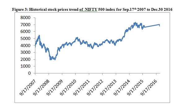
1. Identification stage: In order to forecast stock prices of S&P BSE 500 index and NIFTY 500 index, ARIMA model have been applied. Table1 reports the statistical description for daily observations of S&P BSE 500 and NIFTY 500 stock Index during the period of 1999-2016 that contains; mean, median, max, min, skewness, kurtosis, standard Error and Shapiro-wilk results.

Correlogram Analysis

A correlogram is used to determine whether a particular series is stationary or nonstationary. Usually, a stationary time series will give an autocorrelation function (ACF) and partial autocorrelation function(PACF) that decay rapidly from its initial value of unity at zero lag. In the case of nonstationary time series, the ACF dies out gradually over time. The correlogram of the time series of S&P BSE 500 index and NIFTY 500 index was observed to be nonstationary as the ACF dies down extremely slowly. Differencing is used to make this non stationary time series become stationary. The value of difference (𝑑) is determined by the number of times the differencing is performed on the time series.

Augmented Dickey-Fuller test

The present study employs the Augmented Dickey Fuller test to examine whether the time series properties are stationary or not. The results are present that all series are nonstationary at 1 percent, 5 percent and 10 percent level of significance i.e.,there are unit roots in the time serie. The main result based on this test is that; ADF test is statistically not significant at all level of significance.This indicates to accept null hypothesis and reject that the stock prices are stationery. That all confirms the existence of autocorrelation. Hence the null hypotheses of ADF test are accepted and concluded that the time series data are nonstationary at level.

2.Estimation and diagnostic checking stage

In order to construct the best ARIMA model for S&P BSE 500 and Nifty 500 index, the autoregressive (𝑝) and moving average(𝑞) parameters have to be effectively determined for an effective model. Table 3 shows the different parameters 𝑝 and 𝑞 in the ARIMA model. ARIMA (0, 1, 1) is considered the best for S&P BSE 500 index and ARIMA (2,1,2) is considered the best for NIFTY 500 index is as shown in Table 2 and Table 3.

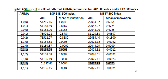
The optimal model order is chosen by the number of model parameters, which minimizes either Akaike Information Criterion (AIC) or Bayesian Information Criterion (BIC).In the process of diagnosis it is verified whether the residual or error generated if white noise or not. The autocorrelations specifying Q*-value, P-value (significance) at different degrees of freedom having a lag of maximum 200 are shown in the table (Table 5). To determine whether the time series is white noise or not, the Ljung-Box Q* statistic is compared with the chi-square distribution with (h-m) degrees of freedom. Here h is the number of lags and m is the number of parameters. Table 5 clearly demonstrates that the Q* statistic has same distribution as chi-square with (h-m) degrees of freedom. Plots and the autocorrelations generated indicated that the model fits well.

Table 5. Ljung-Box test for the Verification of White Noise

3. Forecasting stage:

In forecasting stage, the best model selected can be expressed as follows:

𝑌_t = 𝜙 ₁ 𝑌_t-1 + 𝜃₀ + 𝜀_t,

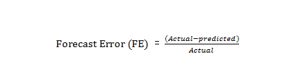
where 𝜀_t = 𝑌_t − is the difference between the actual value and the forecast value of the series

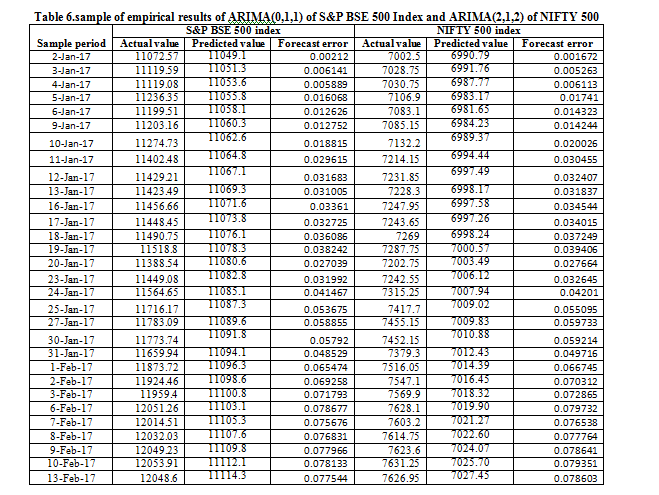
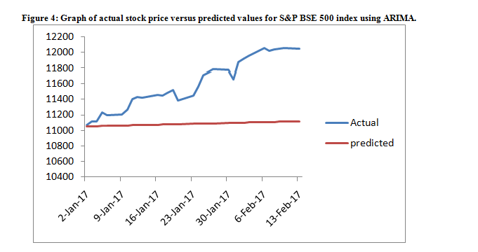
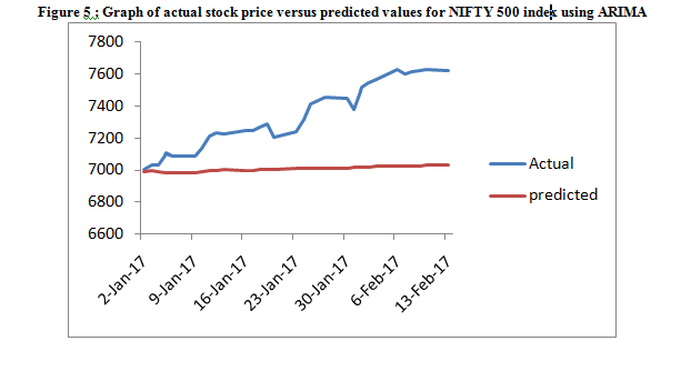
This study experimented with different parameters of autoregressive (𝑝) and moving average (𝑞) in order to determine the best model that will give best forecast as indicated in Table 6.ARIMA (0,1,1) is considered the best for S&P BSE 500 index and ARIMA(2,1,2) is considered the best NIFTY 500 index is as shown in Table 2&3; hence it was selected as the best models based on the criteria listed in the previous section. The actual stock price and predicted values are presented in Table 6, while Figure 4&5 gives the graph of predicted price against actual stock price to see the performance of the ARIMA model selected. However, the forecast error is slightly low and impressive as the predicted values are close to the actual values and move in the direction of the forecast values in many instances as shown in Figure 2, which depicts the correlation of the level of accuracy. The forecast error is determined by

The Box –jenkins methodology used ARIMA model to calculate the errors between the actual close price and the predicted close price generated by all the model. In this study mean square percent error (MSPE) have been used for each method of forecasting and each stock index. The table 7 shows results to find the best model from three models for forecasting of stock prices in Indian stock market is ARIMA. Figure 4 & 5 displays the comparison between the actual close of S&P BSE 500 Index and NIFTY 500 index forecasted close price generated by the ARIMA model discussed above during Jan 2, 2017 to Feb 13, 2017.

Table 7 MAPE from Three forecasting model of the result

Conclusion

In the current research an attempt was made to study whether ARIMA model achieves better results than moving average and Holt & winters exponential methods. The box-jenkins methodology applied ARIMA model to forecast the stock prices for S&P BSE 500 Index and NIFTY 500 Index The analysis of the performance of the Indian stock market with respect to time presents us a suitable time series ARIMA model (0,1,1) and (2,1,2) which helps us in predicting the approximate values of the future. The developed stock price predictive model with the ARIMA indeed, the actual and predicted values of the developed stock price predictive model are slightly close. ARIMA(0,1,1) and ARIMA(2,1,2) as the best model based on the fact that it satisfies all the conditions for the Goodness of Fit. In this study three models were used to apply into two stock market indices in order to find suitable forecasting model which get better error more than currently model . The results showed that the ARIMA model get the best MAPE (Mean Absolute Percentage Error) which is the measurement of this study.

References

1. G.E.P. Box, G. Jenkins, “Time Series Analysis, Forecasting and Control”, Holden-Day,

San Francisco, CA, 1970.

2. Dase R.K. and Pawar D.D., “Application of Artificial Neural Network for stock market predictions: A review of literature” International Journal of Machine Intelligence, ISSN: 0975– 2927, Volume 2, Issue 2, 2010, pp-14-17.

3. JingTao YAO and Chew Lim TAN , “Guidelines for Financial Prediction with Artificial neural networks“.2011
4. David Enke and Suraphan Thawornwong, “The use of data mining and neural networks for forecasting stock market returns, 2005.
5. Abdulsalam sulaiman olaniyi, adewole, kayoed, Jimoh R.G, “Stock Trend Prediction using Regression Analysis – A Data Mining Approach”, AJSS journal, ISSN 2222-9833, 2010.
6. M. Suresh babu, N.Geethanjali and B. Sathyanarayana, “ Forecasting of Indian Stock Market Index Using Data Mining & Artificial Neural Nework”, International journal of advance engineering & application, 2011.
7. Ching-Hsue cheng, Tai-Liang Chen, Liang-Ying Wei, “ A hybrid model based on rough set theory and genetic algorithms for stock price forecasting”, 2010, pp. 1610-1629.
8. Hsien-Lun Wong, Yi-Hsien Tu and Chi-Chen Wang, “Application of fuzzy time series models for forecasting the amount of Taiwan export”, Experts Systems with Applications, 2010, pp. 1456-1470.
9. Assaleh, K. El-Baz, H. and Al-Salkhadi, S. (2011)."Predicting stock prices using polynomial classifiers: The case of Dubai financial market". Journal of Intelligent Learning Systems and Applications, 3: 82-89.

10.Whiteside II PE, J. (2008). "A practical application of Monte Carlo simulation in forecasting". .AACE International Transactions. 4: 1-12.

11. Merh N., Saxena Vinod P., Raj Pardasani K.(2010). “A Comparison between Hybrid Approaches of ANN and ARIMA for Indian Stock Trend Forecasting”. Business Intelligence Journal,july,23-43.
12. Rene D. Estember, Michael John R. Maraña.(2016).Forecasting of Stock Prices Using Brownian Motion – Monte Carlo Simulation. IEOM Society International, March 8-10,704-713.
13. 13. Dima Waleed Hanna Alrabadi , Nada Ibrahim Abu Aljarayesh. (2015). Forecasting Stock Market Returns Via Monte Carlo Simulation: The Case of Amman Stock Exchange. Jordan Journal of Business Administration, Volume 11, No. 3,745-756.
14. Mayankkumar B Patel, Sunil R Yalamalle.(2014). Stock Price Prediction Using Artificial Neural Network .International Journal of Innovative Research in Science,Engineering and Technology, Vol. 3, Issue 6, 13755- 13762.
15. Ayodele Ariyo Adebiyi, Aderemi Oluyinka Adewumi and Charles Korede Ayo(2014). Comparison of ARIMA and Artificial Neural Networks Models for Stock Price Prediction. Journal of Applied Mathematics,vol.2014,1-7.