Pacific B usiness R eview I nternational

A Refereed Monthly International Journal of Management Indexed With THOMSON REUTERS(ESCI)
|
Dr. Padma Kurisetti Associate professor School of Management National Institute of Technology (NIT) Warangal, India |
Swapna Yeldandi MBA School of Management National Institute of Technology (NIT) Warangal, India |
Swamy Perumandla Research Scholar School of Management National Institute of Technology (NIT) Warangal, India |
The main purpose of this paper is to provide insights to the investors and portfolio managers in terms of reducing portfolio risk and enhancing their returns using co integration, Vector Error Correction Model (long and short run relationships) among the selected sectoral indices. It also demonstrates the importance of usage of sector indices which provides insight for sectoral specific investment opportunities and direction for suitable investment decision for the Indian market. The present paper is based on secondary data on the closing prices of the selected sectoral indices from NSE; the span of data is from1stJanuary 2010 to 1 st April 2016. The sectoral indices CNX AUTO, CNX ENERGY, CNX FMCG, CNX IT, CNX PHARMA, and CNX BANK are selected based on market capitalization. We employed the unit root test ADF (Augmented Dickey Fuller Test)and Co- Integration test developed by Engle and Granger (1987),allowing for an unknown number of breaks. The Error Correction Model (ECM) has been used to analyze the long-run and short-run equilibrium relationship among the selected sectoral indices. Our results indicate that there is long run and short run relationship among the sectoral indices.
Keywords: Augmented Dickey Fuller Test, Co Integration, Error Correction Model, Sectoral Indices, and Investment Decisions.
An index is essentially an imaginary portfolio of securities representing a particular market or a proportion of the market. An Index is important to give information about the price movements of products in markets such as the financial, commodities etc. A stock market index is created by selecting a group of stocks that represents the whole market or a specified individual sector or selected segment of the market. An Index is calculated by considering a base period and a base index value. Sectoral indices represent the performance of companies that indicate a movement in specific sector. This is particularly valuable when an index reflects a)highly up-to-date information b) when portfolio of an investor contains illiquid securities. In recent years, indices have come to the lime light to direct applications in finance, in the form of index funds and index derivatives. Index funds are funds in general which are passively invested in the index. Index derivatives allow people to alter their risk exposure either by hedging or by speculation. Index derivatives have become important in risk management especially in the modern economy by using hedging strategy. Finally, indices serve as a benchmark for measuring the performance of fund managers. All-equity fund should obtain returns at least on par with the overall stock market such as NSE or BSE. The sectoral Indices are designed to reflect the behavior and performance of the respective segment of the financial or commodity market etc. The selected Indices are computed by using free float market capitalization method. The level of the index explains the total free float market value of all the stocks in the index with reference to particular base market capitalization value.
Table1
Market Capitalization of Selected Sectoral Indices
|
S.No |
Indices |
No of exchange listed Tradable companies |
Free float market capitalization with NSE(%) |
Free float market capitalization to respective sector (%) |
|
1 2 3 4 5 6 |
Nifty Auto Nifty Bank Nifty Energy Nifty FMCG Nifty IT Nifty Pharma |
15 12 10 15 10 10 |
8.6% 15.6% 11.05% 8.6% 12.15% 6.1 |
91.1% 93.3% 82.65% 80.4% 91.9% 79.9 |
Source: collected and compiled data from NSE official website
The paper is presented as follows. Section 2reviews the related literature. Section 3materials and methods, it presents research methodology and research hypothesis. Section 4 presents the results of co-integration analysis along with results of ADF test, an error correction model and Section 5 presents conclusions.
Chen et al. (1986) analyzed the impact of macroeconomic variables and stock prices. They stated that there is a co-movement of asset prices and macro-economic variables such as interest rates, inflation and industrial production etc. however the exact economic variable impact was not identified. They concluded that stock returns are exposed to systematic economic news. Granger (1987) identified and analyzed set of time-series macro variables and co integrated the relationship of identified macro variables. When they are integrated, in the same order ina linear combination of the variables, it is stationary. He emphasized the use of further factor, ‘equilibrium error’ which arose from the concept of co integration. Thus error correction models should produce short and long run forecasts. Mukherjee and Naka (1995) applied Johansen's (1991)Vector error correction method (VECM) to investigate whether co integration exists between Tokyo stock exchange index and the six Japanese macro-economic variables such as inflation rate, money supply, real economic activity, exchange rate, long-term government bond rate, and call money rate. They explored that co integrating relationship existed and that stock prices are contributed to this relation. The study by Sarkar et al. (2009) focuses on Indian stock market volatility, volatility transmission channels and its response to overseas market indices. The relationship between the SENSEX and various sectoral indices was investigated and it was found that there exists volatility in the developed market indices. A few studies were conducted by (Ewing, 2002; Ewinget al., 2003; Wang et al., 2005)to know the performance of actively managed portfolios by using sector indices as a benchmark tool. Ramin Cooper Maysami & Tiong SimKoh , 2000 examined the long run equilibrium relationship between Singapore stock index and selected macroeconomic variables as well as stock indices of the Singapore, Japan and the United States by using vector error correction model they have suggested that Singapore stock market is interest and exchange rate sensitive. Singapore stock market is significantly and positively co integrated with Japan and the United States stock markets. Demirer and Lien (2005) worked on the correlation between the various sectoral indexes with market movement. The study found that the sectoral correlation is higher in the upside movement of market. Only the finance sector had the strong correlation in the downside market in the context of China market. Philipp Fasnacht & Henri Loeberge (2007) Studied International stock market by using correlations: they used a sectorial approach and they found that sectorial correlations between markets are more stable over time than correlation at the market level and sectorial correlations within countries. Sectors such as Industry, Financials and Consumer services present however a rather high proportion of inconsistent correlation coefficientsParikshit. K. Basu (2008) analysed the importance of industry selection in a portfolio selection.They used a sample of 10 industrial sectors for equity markets in India. They argued that if industry selection is important, the correlations within the industry are important for optimization of portfolio to enhance portfolio returns. Kallberg & Pasquariello (2008) analyzed on the 82 sectoral indices of the US market and had found that there was high correlation between the excess movement in the sectoral indices and there was significance between each other in the movement in a single direction. Patra & Poshakwale (2008) found that there was low relation in the sectoral returns in the long run. However there was an impact of the banking sector on the other sector indices return and variance. This research paper suggested that the changes and information of the banking sector could be used in order to predict the returns of the other sectoral indices in short term. Pyeman and Ahmad (2009) study long and short-run relationships between sectoral indices and macroeconomic variables with reference to Malaysia. Trends in macroeconomic variables such as real economic activity, rate of interest, rate of inflation, supply of money and exchange rate results in varied responses from sectorial indices. Unanticipated changes in macroeconomic variables result in different levels of speed adjustments towards long-run equilibrium among various sectors. An attempt was made by Piyush Kumar Singh & Venkata Vijay Kumar (2011) to analyze the movement of sectoral returns and their contributions towards the BSE Sensex returns. The study found that the BSE Sensex returns could be explained with the help of selected sectoral index returns. The study aimed at the short and long run relationships of BSE (BSE 500, BSE 200, and BSE 100) and crude price by Bhunia, A. (2012). Shanmuga sundram and Benedict (2013) the study attempts to find out the volatility of the Indian sectorial indices. ANOVA & t-test were used to indentify the differenceof risk factor among the sectorial indices and Nifty. Study found that there is no difference in the standard deviation among various sectorial indices & there is a difference in the mean scores of various time intervals. S. kirithiga, Dr. R. Azhagaiah(2014), the study analyzed the linkage among various agricultural commodities and their cross hedging possibility in India. The study was based on secondary data collected from National Commodity and Derivative Exchange (NCDEX). The relationship among these agricultural commodities is tested by using Error Correction Model (ECM). The results obtained reveal that there exist short run and long run equilibrium relationships among these agricultural commodities. Dhungel (2014) has applied Error Correction Model (ECM) to investigate the short and long run equilibrium by considering the secondary data of electricity consumption in Nepal from 1974 to 2011. In his model he had used electricity consumption as dependent variable, foreign aid and GDP as explanatory variables. The results of ECM indicate that there exists both short- and long-run equilibrium in the system. Anpukarasi and Nithya (2014)have examined return and volatility across the 11 sectoral indices and CNX NIFTY index. The study found that the correlation among most of the indices is significant.The study was conducted by collecting the data from the period 02.04.2001 to 31.03.2011. The study concluded that there was a co integrated long run relationship between BSE (BSE 500, BSE 200, and BSE 100) and crude price. Granger causality results reveals that there was one way causality relationship between BSE (BSE 500, BSE 200, BSE 100) and crude price but not vice versa. Mei-Se Chien et al (2015) examines the dynamic process of convergence among cross-border stock markets in China and ASEAN-5 countries using recursive co-integration analysis. Their results show that these six stock markets had at most one co-integrating vector from 1994 to 2002. Overall, the regional financial integration between China and ASEAN-5 has gradually increased. Additionally, the estimated coefficients of error correction terms are statistically significant and negative in China and Indonesia, but the coefficients of other countries are insignificant, meaning that all of the adjustment of this co-integration fell on these two countries' stock markets. Sajal Ghosh & Kakali Kanjilal . (2016) analyzed the co-integration among oil prices, exchange rate and Indian market is examined threshold co-integration tests are employed to analyse the data. Indian stock market becomes integrated with the international events 2009 onwards.
1. Objectives of the Study
1. To find the index based investment opportunities of selected sectoral indices and their movements.
2. To investigate the long-run and short-run equilibrium relationships of the selected sectoral indices.
2. Methods of Data Collection and Sampling Design
The present study is based on the secondary data. The data have been collected from monthly reports of identified sectorial indices (CNX Auto, CNX Bank, CNX Energy, CNX FMCG, CNX IT, and CNX Pharma).The study period is from January 1, 2010 to April 1, 2016. The daily closing prices of the indices have been considered for the analysis.
3. Research Tools and Methodology
The Augmented Dickey-Fuller (ADF) - Unit Root Test:
ADF is the augmented form of Dickey Fuller Test. This test is used for checking the presence of unit root. ADF is used for complicated time series data. ADF is used in following type of models: ∆𝑦𝑡 = 𝛼 + 𝛽𝑡 + 𝛾𝑦𝑡−1 + 𝛿1∆𝑦𝑡−1 + ⋯ + 𝛿𝑝∆𝑦𝑡−𝑝 + 𝜀𝑡 ….(1)Where 𝛼 is a constant, 𝛽 is coefficient of time trend and p is the lag order of autoregressive process. This means that ADF allows high order autoregressive processes. To find which order to use in ADF, either regression or alternatively any of the information criterion like Akaike Information Criterion (AIC), Schwarz information criterion(SIC) or Hannan Quinn information criterion (HIC). Unit root test hypothesis is 𝐻0: 𝛾 = 0 Unit Root Present𝐻0: 𝛾< 0 No Unit Root.
Co integration Theory and Engle Granger Co integration Test:
Two series are said to be co integrated if they have unit root present individually in each of them and their linear combination has lower order of integration. This theory was developed first by Engle and Granger (1987). If we have 𝑥t and 𝑦t as non-stationary series of I (1) and on regressing 𝑦t on 𝑥t: 𝑦t = 𝑥t + 𝜀t. If 𝜀t ~ I(0) …(1)then these two series are said to be co integrated of order one. This is precisely the Engle Granger Test. Engle Granger Co integration technique firstly requires a Unit Root Test to check whether the considered series are stationary or not. This unit root test can be performed using Augmented Dickey Fuller or Philips Perron (PP) test. Co integration technique is used to find long term relationship between the selected sectoral indices. Once the stationarity is verified, co integration test is conducted to check which indices are co integrated and have equilibrium relation with the dependent index. An error correction model (ECM)belongs to a category of multiple time series models most commonly used for data where the underlying variables have a long-run stochastic trend, also known as co integration . ECMs are a theoretically-driven approach useful for estimating both short-term and long-term effects of one time series on another. The term error-correction relates to the fact that last-periods deviation from a long-run equilibrium, the error, influences its short-run dynamics. Thus ECMs directly estimate the speed at which a dependent variable returns to equilibrium after a change in other variables. Several methods are known in the literature for estimating this model. Among these Engel and Granger 2-step approach is used in this study.
Engel and Granger 2-Step Approach
The first step of this method is to pretest the individual time series one uses in order to confirm that they are non-stationary in the first place. This can be done by standard unit–root testing such as Augmented Dickey–Fuller test . Take the case of two different series {\displaystyle x_{t}}and {\displaystyle y_{t}}if both are I (0), standard regression analysis will be valid. If they are integrated of a different order, e.g. one being I (1) and the other being I (0), one has to transform the model. If they are both integrated to the same order (commonly I (1)), we can estimate an ECM model of the form:
 …(2)
…(2)
If both variables are integrated and this ECM exists, they are co integrated by
the Engle-Granger representation theorem. The second step is then to estimate the
model using Ordinary least squares . {\displaystyle y_{t}=\beta _{0}+\beta _{1}x_{t}+\epsilon
_{t}}If the regression is not spurious as determined by test criteria described
above, Ordinary least squares will not only be valid, but in fact super consistent
(Stock, 1987). Then the predicted residuals {\displaystyle {\hat {\epsilon _{t}}}=y_{t}-\beta
_{0}-\beta _{1}x_{t}} from this regression are saved and used in a regression of
differenced variables plus a lagged error term
…. (3) {\displaystyle A(L)\Delta y_{t}=\gamma +B(L)\Delta x_{t}+\alpha {\hat {\epsilon
_{t-1}}}+\nu _{t}} One can then test for co integration using a standard t-statistic
on α. {\displaystyle \alpha }The results of ECM to find the short-run and long-run
equilibrium relations are depicted in Table No.6: The choice of lag lengths may
be decided using Sim’s likelihood ratio test. However, for simplicity, in this article
we have used the multivariate forms of the Akaike Information Criterion (AIC) and
Schwartz Bayesian Criterion (SBC), where AIC =T ln (residual sum of squares)+2nand
SBC=T ln (residual sum of squares) + n ln (T).
4. Hypothesis
To analyze the first objective of the study i.e., to find the index based investment opportunities of selected sectoral indices and their movements, the following hypotheses are made.
. H 01 “The prices of the selected sectorial indices dealt in NSE move independently”.
. H02 “There is no co integration exists among the selected sectoral indices.
. H03 “There is no long-term equilibrium relationship exists among the prices of selected sectorial indices dealt in NSE”.
. H04 “There is no short-run equilibrium relationship exists among the prices of selected sectoral indices dealt in NSE”.
5. limitation and scope of the study:
The study covers the selected indices prices of sectoral indices traded in NSE for the study period. The study is based on secondary data therefore the quality of the study depends purely upon the accuracy, reliability and the quality of the secondary data source. The findings of the study might differ if considering the data from other stock exchanges from India or elsewhere. Hence studies considering other exchanges and other indices can also be done by focusing on various macroeconomic factors.
The analysis of the study has been divided into two parts. The first part of the analysis is deals with the study of descriptive statistics and correlations of selected sectoral indices prices and the second part of the analysis focuses on the ADF, co-integration and ECM (Short Run and Long Run equilibrium).
Results of Descriptive Statistics
The data which is collected from the closing prices of selected sectoral indices of NSE, has been analyzed using descriptive statistics(Mean, Standard Deviation, Skweness, Kurtosis and Jarque Bera). The results of the same are compiled and arranged in Table No.2.
Table 2:
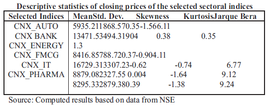
Results of descriptive statistics analysis reveals that the mean of the selected sectorial indices for the study period (Jan 2010 to April 2016) represents that CNX FMCG has highest mean(16729.31) and mean of CNX AUTO is lowest (5935.21), which means that there is high price differential among the prices of identified sectoral indices. The standard deviation which measures the deviation from mean values represents that CNX ENERGY has lowest standard deviation (788.72) and CNX BANK (3494.31) has highest standard deviation.This shows that CNX BANK is highly volatile and has high levels of risk where as CNX ENERGY is less volatile and low risky. Jarque Bera statistics reveal that all the selected indices are not normally distributed except CNX ENERGY and CNX BANK. However, with descriptive statistics we could not finalize and conclude any results hence a further analysis of correlation has been conducted.
Correlation Analysis
According to the modern portfolio theory, if an investor wants to retain the yield at the same level and reduce the variance/risk by decentralized investment, investor is expected to select the securities which are not perfectly positively correlated. Theoretically, the non-systematic risk can be reduced to zero by fully diversified investment. With the influence of this theory, many research studies concentrated on correlations among stocks or stock groups, mainly on correlations between stock markets of different regions, different styles or different sectors. The correlation among the stocks affect the investor's investment risk and return, and help investors better understand and evaluate India’s securities objectively. The correlation analysis have been conducted on the selected six sectoral indices and the results are compiled in Table No.3
Table 3:
Correlation among the closing prices of the selected sectorial indices
| INDICES | CNXAUTO | CNXBANK | CNXENERGY | CNXFMCG | CNXIT | CNX PHARMA |
| CNX AUTO | 1 | 0.97 | 0.66 | 0.89 | 0.94 | 0.97 |
| CNX BANK | 0.97 | 1 | 0.67 | 0.84 | 0.85 | 0.92 |
| CNX ENERGY | 0.66 | 0.67 | 1 | 0.56 | 0.57 | 0.51 |
| CNX FMCG | 0.89 | 0.84 | 0.56 | 1 | 0.88 | 0.90 |
| CNX IT | 0.94 | 0.85 | 0.57 | 0.88 | 1 | 0.95 |
| CNX PHARMA | 0.97 | 0.92 | 0.51 | 0.90 | 0.95 | 1 |
Source: Computed results based on data collected from NSE
Interpretations:
A highest positive correlation was observed between the closing prices of CNX AUTO and CNX PHARMA(0.97),CNX BANK(0.97), followed by CNX IT(0.94), CNX FMCG(0.89). But CNX ENERGY(0.66) is less correlated with CNX AUTO. CNX BANK is possitively highly correlated with CNX PHARMA(0.92),CNX IT(0.85), and CNX FMCG(0.84), but CNX BANK is less correlated with CNX ENERGY(0.67). CNX ENERGY has a low correlation with all other indices CNX FMCG has a high possitive correlation with CNX PHARMA and CNX IT. CNX IT also has high positive correlation with CNX PHARMA.
Based on the correlation analysis it is observed that there is ahigh positive correlation between the sectoral indices except CNX ENERGY. These results disprove the hypothis that H01 “The prices of the selected sectorial indices dealt in NSE move independently”. This analysis will provide the investor and portfolio manager an idea regarding the correlated sectors among the selected secor indices . However, the results of correlations among the indices maynot provide the sufficient implications towards the investment decisions. Hence a further analysis of co integration is done to find long and short run relationship among indices. Incase of time series data to conduct the co integration another test was applied to check whether the data is stationary or not. Co integration test can be applied only if the data is stationary.To check whether the data is stationary or not, ADF on prices of indices has been conducted(unit root test).
To provide a further insight to investors as well as portfolio managers second objective has been analysed ,i.e., to investigate the long-run and short-run equilibrium relationships of the selected sectoral indices. The hypotheses H03, H04are analyzed by using ADF test for unit root, ADF test on residuals to check the spurious regression, Co integration test, ECM and ECT to find long and short run equilibrium relationship.
The finding of the ADF test exhibits that all indices are non-stationary in their level. However, stationarity is found after first difference. It indicates that they are in the same order that is I(1). It is the fundamental criteria to examine the long run relationship between the indices. The ADF test results estimated using equation (1) are given in Table No.4.The null hypothesis of a unit root is rejected in favor of the stationary alternative in each case if the test statistic is more negative than the critical value.
Table 4
ADF Test for stationarity
|
SECTORAL INDICIES |
First difference |
|
|
T stat for constant and trend |
P -value |
|
|
CNX AUTO CNX Energy CNX FMCG CNX IT CNX Pharma CNX PSU BANK |
-2.0 -8.6 -3.0 -11.7 -2.9 -3.2 |
2.1% 0.0% 0.1% 0.0% 0.2% 0.1% |
Source: Computed results(Critical Values at 5% significance)
ADF on Residuals - Spurious regression:
In the study,Agumented Dikney Fuller test on residualsisemployedto check the data for spurious regression. The test suggested that the time series is non stationary at level but stationary at first difference. Hence the series can be checked for co integration. Since the absolute values of t-statistics CNX AUTO(4.997153),CNX Energy(-4.003790),CNX FMCG (-4.298611), CNX IT(-4.034046), CNX Pharma (-4.755567) and CNX Bank (-4.679156)are more than the critical value Engle granger at 10% which is 3.04. Hence the study reject H0 and accept Ha that U(the residuals of the model) does not have Unit root. i.e., U is stationary. Estimated model is non spurious and employed regression model as the residual of the model is stationary.
Table 5
ADF on Residuals: (Checking for Spurious regression):
|
Indcies |
Significance level |
||
|
t-static |
P-Value* |
AIC |
|
|
CNX AUTO CNX Energy CNX FMCG CNX IT CNX pharma CNX Bank |
-4.997153 -4.003790 -4.298611 -4.034046 -4.755567 -4.679156 |
0.0001 0.0029 0.0012 0.0027 0.0003 0.0004 |
13.50998 14.45708 15.99961 15.17441 14.88784 13.58053 |
Source: Complied results in Eviews based on data collected from NSE
*One sided p-values @5% Significance level.
Co integration Results
Cointegration analysis allows non stationary data to be used so that spurious results are avoided. It also provides applied econometricians an effective formal framework for testing and estimating long-run models from actual time-series data.
Table 6: Co integration results using ECM
|
INDICES |
CNX Auto co integration with other indices Coefficient Std. Error T Statistic Prob.* |
|||
|
CNX ENERGY CNX IT CNX PHARMA CNX BANK |
0.230392 0.190566 0.398816 0.593201 |
0.074920 0.049164 0.044276 0.083872 |
3.075154 3.876131 9.007591 7.072694 |
0.0035* 0.0003* 0.0000* 0.0000* |
|
CNX Energy co integration with other indices |
||||
|
CNX AUTO` CNX FMCG` CNX PHARMA |
0.740140 0.086821 -0.500386 |
0.240684 0.042635 0.109372 |
3.075154 2.036364 -4.575053 |
0.0035* 0.0475* 0.0000* |
|
CNX FMCG co integration with other indices |
||||
|
CNX ENERGY CNX BANK |
0.952450 -1.565673 |
0.467721 0.681334 |
2.036364 -2.297951 |
0.0475* 0.0262* |
|
CNX IT co integration with other indices |
||||
|
CNX AUTO CNX BANK |
1.291956 -1.191534 |
0.333311 0.262085 |
3.876131 -4.546358 |
0.0003* 0.0000* |
|
CNX Pharma co integration with other indices |
||||
|
CNX AUTO CNX ENERGY CNX BANK |
1.600198 -0.624969 -0.666236 |
0.177650 0.136604 0.221967 |
9.007591 -4.575053 -3.001513 |
0.0000* 0.0000* 0.0043* |
|
CNX BANK co integration with other indices |
||||
|
CNX AUTO CNX FMCG CNX IT CNX PHARMA |
0.878198 -0.065770 -0.260192 -0.245820 |
0.124167 0.028621 0.057231 0.081899 |
7.072694 -2.297951 -4.546358 -3.001513 |
0.0000* 0.0262* 0.0000* 0.0043* |
The above table is compiled based on the co-integration results the probability (*) value where less than 5%.
After checking the co-integration among the all sectoral indices we observed that
· CNX Auto is co integrated with CNX Energy, CNX IT, CNX Pharma and CNX Bank,
· CNX Energy is co integrated with CNX Auto, CNX FMCG, and CNX Pharma.
· CNX FMCG is co integrated with CNX ENERGY and CNX BANK.
· CNX IT is co integrated CNX Auto and CNX Bank.
· CNX Pharma is co integrated CNX Auto, CNX Energy and CNX Bank .
· CNX Bank is co integrated with CNX Auto, CNX FMCG, CNX IT and CNX Pharma.
The cointegration shows that which explains long-run equlibrium relationship among the response and predicator variable there by rejecting the H03, i.e., “There is no cointegration among the prices of selected sectoral indices dealt in NSE”. That means they have long run equilibrium relation. As the variables are co integrated so we can run ECM model. That means they have long run equilibrium relation.
ErrorCorrection term of ECM of long-run Equilibrium relation.
The analysis of ECM are presented in the Table No.7 shows that the Error Correction Terms (ECT) are negative and significant, which explains long-run equlibrium relationship among the response and predicator variable there by rejecting the H03, i.e., “There is no long-term equilibrium relationship among the prices of selected sectorial indices dealt in NSE”. The ECT of CNX AUTO is negative (-0.53,Table no.) and is significant at 1% level, meaning that system corrects its previous priod disequilibrium at a speed of 53.5% annually. So, the long term investors can keep hope in case of unfavourable situations as the sector moves to equilibrium at a speed of 53.5%.The ECT of CNX ENERGY is negative (-0.46,Table no7.) and is significant at 1% level, meaning that system corrects its previous priod disequilibrium at a speed of 46.4% annually.The ECT of CNX FMCG is negative (-0.16,Table no.) and is significant at 1% level, meaning that system corrects its previous priod disequilibrium at a speed of 16% annually. CNX FMCG that covers day to day needs of individuals, there are less chances of this index being moving down.The ECT of CNX IT is negative (-0.42,Table no.) and is significant at 1% level, meaning that system corrects its previous priod disequilibrium at a speed of 42% annually. So, the long term investors can keep hope in case of unfavourable situations as the sector moves to equilibrium at a speed of 42%.The ECT of CNX PHARMA is negative (-0.50,Table no.) and is significant at 1% level, meaning that system corrects its previous priod disequilibrium at a speed of 50% annually. So, the long term investors can keep hope in case of unfavourable situations as the sector moves to equilibrium at a speed of 50%.
Table 7
Error Correction term of ECM of long-run Equilibrium relation
|
Index |
Co efficient t-static Probability |
|
CNX AUTO ECT CNX ENERGY ECT CNX FMCG ECT CNX IT ECT CNX PHARMA ECT CNX BANK ECT |
-0.535383-3.557450 0.0009* -0.464467-3.601385 0.0008* -0.159078-2.158863 0.0006* -0.420006-3.723689 0.0005* -0.503969-3.8636304 0.0003* -0.427983-3.571959 0.0009* |
*significant at 1% level, **Significant at 5% level, ***significant at 10% level
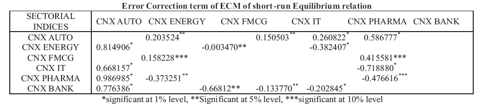
Error Correction term of ECM of short-run Equilibrium relation
ECM explains short-run equlibrium relationship when the lagged values of the response and predicator variables are significant there by rejecting the H04, i.e., “There is no short-run equilibrium relationship among the prices of selected sectorial indices dealt in NSE” .CNX AUTO has a positive short run equilibrium relation with CNX ENERGY(0.20), CNX IT(0.15), CNX PHARMA(0.26) , CNX BANK(0.59) and has no relation with CNX FMCG. Hence , investor can take decisions based on these results.CNX ENERGY has a positive short run equilibrium relation with CNX AUTO(0.81) negative short run equilibrium relation with CNX FMCG (-0.003),CNX PHARMA(-0.38) and has no relation with CNX IT and CNX BANK. CNX FMCG has a positive short run equilibrium relation with CNX ENERGY(0.16) and CNX BANK(0.42) and has no relation with CNX AUTO, CNX IT, CNX PHARMA. CNX IT has a positive short run equilibrium relation with CNX AUTO(0.67)and negative short run equilibrium relation with CNX PHARMA(-0.72) and has no short run equilibrium relation with CNX ENERGY, CNX FMCG and CNX PHARMA.CNX PHARMA has highest positive short run equilibrium relation with CNX AUTO(0.78) and negative short run equilibrium relation with CNX ENERGY(-0.37), CNX BANK(-0.48) and has no relation with CNX FMCG and CNX IT.CNX BANK has a positive short run equilibrium relation with CNX AUTO(0.78) ,CNX FMCG, CNX IT , negative short run equilibrium relation with CNX PHARMA and has no relation with and CNX BANK.
Table 8
In this work we explored co integration, long and short run equilibrium among the considered six indices. Based on these emperical results investors and portfolio managers can take specific sector based strategic portfolio decisions.Many people believe that if you pick the fastest growing sector or sectors in which to invest, you get a leg up on the investing competition and can outperform the general markets. We explore sector index investing and give you some information to help investors to decide that whether to tilt your investment portfolio towards certain sectors or maintain a broad based investing approach. While our analysis also explored co integrated sectoral indices and their equilibriums in terms of long and short run. Hence these results explore important implications to investors and portfolio managers in terms of reducing portfolio risk and enhancing their returns. In this study we have investigated the correlation co integration and long and short run equilibrium relationships among the identified sectoral indices but the reasons should be traced out in further study in this connection.
Amalendu Bhunia. (2012). Cointegration and Causal Relationship among Crude Price, Domestic Gold Price and Financial Variables: An Evidence of BSE and NSE , Journal of contemporary issues in business research, vol (2), I, pp01-10.
Amitava Sarkar Gagari Chakrabarti and Chitrakalpa Sen .(2009).Indian stock market volatility in recent years: Transmission from global market, regional market and traditional domestic sectors, Journal of Asset Management 10(1) ·
Ang,Andrew, Robert Hodrick, Yuhang Xing, and Xiaoyan Zhang. (2006). The Cross-Section of Volatility and Expected Returns, Journal of Finance , vol. 61(1) (February): 259–299.
Charles Adjasi, Simon K. Harvey, Daniel Agyapong. (2008). Effect of Exchange Rate Volatility on the Ghana Stock Exchange, African Journal of Accounting, Economics , Finance and Banking Research, Vol. 3. No. 3.
Dr. M. Anbukarasi and B. Nithya.(2014). Return and Volatility Analysis of the Indian Sectoral Indices- with special reference to National Stock Exchange, EPRA international Journal of Economic & Business Review, Vol. 2, Issue – 8, pp 90-97.
Nai Fu Chen, Richard Roll and Stephen Ross.(1986). Economic Forces and the stock market, The Journal of Business , Vol. 59, No. 3 383-403.
Demirer, R., Lien, D., & Shaffer, D. (2005). Comparisons of short and long hedge performance: The case of Taiwan, Journal of Multinational Financial Management , 15, 51-66.
Engle, R. F., & Granger, C. W. J. (1987). Co-integration and error correction: Representation, estimation, and testing. Econometrica, 55, 251–276.
Ewing, B. T. (2002), The transmission of shocks among S&P indexes, Applied Financial Economics , 12, 285-290.
Ewing, B. T., Forbes, S. M. and Paye, J. E. (2003), The effect of macroeconomic shocks on sector-specific returns, Applied Economics , 35, 201-207.
Feng Wu, Robert J. Myers. (2011).Volatility spillover effects and Cross Hedging in corn and crude oil futures, Journal of Futures Markets , Volume 31, Issue 11, November.
Jaafar Pyeman, Ismail Ahmad.(2009). Dynamic Relationship Between Sector-Specific Indices And Macroeconomic Fundamentals. , Malaysian accounting review, vol 8(1).
Jarl Kallberg & Paolo Pasquariello. (2008).Time-series and cross-sectional excess co movement in stock indexes, Journal of Empirical Finance, 15 , 481–502
Johansen, Soren.(1988). Statistical analysis of co integration vectors, Journal of Economic Dynamics and Control, Elsevier, vol. 12(2-3), pp. 231-254.
Kamal Raj Dhungel. 2014. On the Relationship between Electricity Consumption and Selected Macroeconomic Variables: Empirical Evidence from Nepal, Modern Economy, 5, 360-366.
Kwon, C.S. and T.S. Shin. (1999). Co integration and causality between macroeconomic variables and stock market returns, Global Finance Journal ,10(1): p. 71.
Mei-Se Chien, Chien-Chiang, Lee Te-Chung Hu , and Hui-Ting Hu . (2015). Dynamic Asian stock market convergence: Evidence from dynamic cointegration analysis among China and ASEAN-5, Economic Modelling , Volume 51 , Pages 84-98.
Mukherjee. T.K. and Naka. (1995). Dynamic Relations between the Macroeconomic Variables and the Japanes Stock Market- An Application of a Vector Error Correction Model, Journal of Empirical resea rch, 18, 223-237.
Parikshit K Basu & Rakesh Gupta,(2009). Sector analysis and portfolio optimization: The Indian experience , International Business & Economics Research Journal. Vol 8 (1).
Patra, T. and S. Poshakwale.(2006). Economic variables and stock market returns: evidence from the Athens stock exchange. Applied Financial Economics , 16(13): p. 993-1005.
Philipp Fasnacht & Henri Loeberge. (2007). International Stock Market correlations: A Sectorial Approach, Finance International Meeting AFFI-EUROFIDAI, Paris , December’ 2007 Paper.
Pyeman, J., and Ahmad, I. (2009). Dynamic Relationship between Sector Specific Indices and Macroeconomic Fundamentals, Malaysian Accounting Review , 8,81-100.
Ramin Cooper Maysami & Tiong Sim Koh . (2000).A vector error correction model of the Singapore stock market, International Review of Economics & Finance . vol 9(1) p.79-96.
Sajal Ghosh and Kakali Kanjilal . (2016). Co-movement of international crude oil price and Indian stock market: Evidences from nonlinear co-integration tests, Energy Economics , Volume 53 , Pages 111-117.
S. kirithiga & Dr. R. Azhagaiah, (2014), Price Spread among the Indian Agricultural Commodity Futures. Pacific Business Review International .vol 7(4) p.48-56.
Dr. G. Shanmuga sundram & D. John Benedict. (2013).Volatility Of The Indian Sectoral Indices - A Study With Reference To National Stock Exchange , International Journal of Marketing, Financial Services & Management Research, Vol.2, No. 8.
Wang, Z., Kutan A. and Yang, J. (2005). Information flows within and across sectors in Chinese stock markets, The Quarterly Review of Economics and Finance, 45, 767-780.