Editorial Board

A Refereed Monthly International Journal of Management

An Evaluation of Pairs Trading Strategy: A Study of Global Currencies

Author

V. HarshithaMoulya Dept. of Business Administration, Mangalore University, Mangalagangothri, Karnataka

Abuzar Mohammadi Dept. of Business Administration Mangalore University, Mangalagangothri, Karnataka

Dr. T. Mallikarjunappa, Professor, Dept. of Business Administration Mangalore University, Mangalagangothri, Karnataka

Abstract

Currency trading market dominates the exchange-based trading market globally in terms of trade volume and value. The cues and shocks to the tightly integrated economies often institute short-term disequilibrium in the long-run relationship of currencies. The arbitrage trading market mechanism prevalent in an efficient market eventually corrects the disequilibrium in the currencies. We studied the co-integration and the mean-reversion in 20 international currencies, and found the cointegration in 39 currency pairs out of 139 pairs analysed. The back-testing procedure of the statistical arbitrage trading showed that the pairs trading strategy on currencies yielded positive arbitrage returns.

Keywords: Currency pairs trading, statistical arbitrage trading, cointegration, global currencies, currency trading

1.Introduction

The pairs trading is a famous Wall Street strategy pioneered by Mr Nunzio Tartaglia during the 1980s(Vidyamurthy,2004)to trade the closely movingpairs of financial assetswheneveran anomaly existed in their relationship. The idea of pairs trading believes in the intuition of mean-reversion to equilibrium and the propositions of the market efficiency. While the efficient market hypothesis (EMH) proposes no scope for abnormal returns, the drivers of market inefficiency create many opportunities for arbitragers for earning a profit. Pairs trading involves taking the short position in the overly priced security and long-position in the under-priced security that has a broader spread, at a pre-determined ratio. The strategy earns a positive arbitrage return when the spread between the securities narrows to an equilibrium value. The pairs trading strategy is prevalent among practitioners. However, it has not attracted much of academic attention (Jacobs and Weber, 2015; Galeshchuk, 2017; Galeshchuk & Mukherjee, 2017). The currency market is sizably bigger thanthe equities and the commodities markets combined. A Bloomberg report of 2012-13 reported that currency market stands as the world’s largest market with a $5.2 trillion in daily trading volume, driven by fundamentals. The Reserve Bank of India (RBI) permitted the currency trading in India in August 2008 by allowing a few currencies to be traded on the NSE platform viz., USD, EUR, GBP and JPY. The currencies traded on the NSE are benchmarked against Indian currency (INR). The RBI report (RBI, 2015) mentioned that the exchange-based trading permitted trading of cross-currency futures and options for EUR-USD, GBP-USD and USD-JPY on the NSE. The derivatives trading in currency futures preceded the currency options for the Indian market. The currency options for USD-INR was introduced in October 2010. In our study, we study the cointegration between currencies of 20 international markets involving the American market, the EU, Australia and several Asian economies. We performed the cointegration analysis on 136 currency pairs and found that 39 shared the long-run equilibrium relationship. We performed the rule-based statistical arbitrage trading on the currency pairs under the pairs trading framework. The back-testing procedure implemented the trading technique based on the trade signals generated to trade the spread between the currency pair. We found that currency pairs trading generated positive arbitrage returns for CNY-PHP, CAD-SEK, and AUD-MYR. We used several evaluation metrics to arrive the profitable currency pairs. The study assumes scope and importance for investors, arbitragers, currency traders and regulators by providing useful insights on the potentially tradable currency pairs for arbitrage returns. The pairs identified reciprocate the economic nexus between the advanced economies and the emerging economies.

Literature Review

Market efficiency and currency trading

Concerning the market efficiency hypothesis and the currency exchange rates, Frenkel and Levich (1977) found no arbitrage opportunity existed for covered interest arbitrage. Hansen and Hodrick(1980) examined whether there is any relation between the expected rate of return in the spot market and the speculation in forward currency rates, and found results contradictory to the hypothesis. The study rejected the market efficiency hypothesis as the findings supported several alternative hypotheses to market efficiency. Fama (1984) studied the predictability of forward exchange rates in forecasting future spot exchange rates and found that both were time dependent. The forward rate premium was negatively correlated with the expected future spot rate estimated using forward rates. The existence of forward premiums established the proposition of Shleifer and Vishny(1997) that arbitrage failed to correct the mispricing in the securities leading to an anomaly due to the limitation of the arbitrage and that markets are not efficient. The following studies contradicted the proposition of market efficiency theory in currency trading. Chaboud, Chernenko and Wright(2008)studied the price behaviour and volume behaviour of EUR-USD and USD-JPY spots in response to announcement of macroeconomic news of the US market, and found spikes in trade volume, negative correlation between the trade volumes the market expectation following the announcements, and the price response preceded a significant surge in trade volume. Röthig (2012) studied short-run causal relationship between speculative trading for currencies and found a significant feedback effect and impulse response for the cross-market herding of the Canadian dollar, Swiss franc, British pound, and Japanese yen futures. Choi(2011) studied arbitrage opportunities in foreign exchange rate using a triangular foreign exchange trading and found that bilateral exchange rate diverged from common currency of a trilateral basket rate yielding arbitrage profit until market attains an equilibrium. Concerning the co-movement among currencies, they found an inverse relationship between the correlation of currencies and their volatilities. Neely and Weller(2013) investigated optimal trading strategies based on technical rules, under the propositions of adaptive markets hypothesis, using the forex rates of the major markets and emerging markets and the data of US equities of S&P500. They found that forex trading outperformed S&P500with larger Sharpe ratios. However, they found no coordination between forex and equity strategies for comparison. They found significant trading-rule returns for forex in emerging markets. Auld and Linton (2019) studied convergence in prices of GBP/USD exchange rate on 24/06/2016,i.e., the EU referendum day and found highly profitable arbitrage opportunities between the two currency markets.

Definition of pairs trading

The pairs trading strategy is the brainchild of the Wall Street quantitative traders. Vidyamurthy (2004)defined pairs trading as the process of identifying pairs of securities that share similar characteristics and have co-movement, followed by trading in the securities whenever an anomaly existed in the relationship to make a profit, with the intuition that the mispricing corrects itself in the long run. Elliott, der Hoek and Malcolm (2005) outlined pairs trading as the technique of trading of similar securities that are out of equilibrium value. The spread measures the relative mispricing in the securities. The higher is the spread, and the greater is the degree of mispricing and the profit potential (Vidyamurthy, 2004). An arbitrage trade of shorting the high-priced security and longing the low-priced security that has a broader spread, at a pre-determined ratio, leads to earninga profit when the spread narrows to some equilibrium value. The ratio of stocks selection for trading the spread portfolio has a beta value zero concerning the market portfolio (Elliott et al., 2005).Chen and Lin(2017) described pairs trading as a strategy of trading relatively correlated assets with dissimilar valuations until the value of the spread between the two assets converges to zero.

The pairs trading framework

Krauss (2017) reviewed the available literature on the relative value arbitrage strategies on securities and found that the studies used non-parametric distance metrics for identifying the potential pairs for trading; co-integration approach for estimation of stationary and mean-reverting spread; stochastic control approach for optimal portfolio holding of pairs. Elliott et al. (2005) provided a framework for implementation of the pairs trading strategy for any financial asset pairs using simulation techniques and obtained parameters that had convergence with the EM algorithm. Adoption of machine learning techniques for the prediction of the currency exchange rates has higher accuracy of prediction and direction of change in returns, thus provides a greater probability of earning an excess return. It was found that the currency traders who leveraged on technology for trading strategies earned profit from the arbitrage opportunities for EUR/USD, the GBP/USD and the USD/JPY currency pairs (Galeshchuk, 2017; Galeshchuk & Mukherjee, 2017). Chen and Lin (2017) discussed two methods for identifying the potential pairs of stocks viz., the minimum squared distance (MSD method) and the fundamental aspects of firms. The MSD method identifies highly correlated stocks with similar systematic risks by measuring the minimum sum squared deviations between two normalised stock prices, whereas, the firms’ fundamentals or industry characteristics identify firms that are exposed to the same risk factors. They used the MSD based on rolling-window approach and the non-parametric methods for calibrating the tolerance level or threshold for trading entry and exit signals of US securities pairs and found that both MSD and the non-parametric methods generated positive excess returns. The threshold or tolerance level detects the potential arbitrage trading opportunities. Gatev, Goetzmann,and Rouwenhorst (2006) had used the MSD method to identify stock pairs. They attributed the abnormal returns from pairs trading to a common factor in returns of the close substitutes. Concerning the estimation of the spread, Elliott et al. (2005) proposed a mean-reverting Gaussian Markov chain model for estimation of the spread. The central idea of pairs trading is to follow the contrarian strategy for trading the spread. An investor should enter into a long (short) position in the spread portfolio when the actual value of the spread is larger (smaller) than the predicted threshold value. The contrarian strategy is applied when the spread reverts to an equilibrium value to earn a profit. Avellaneda and Lee(2010) used the principal component analysis (PCA) and regression techniques for estimation and trading of the spread and applied contrarian strategies in the back-testing process to trade US equity pairs, and found higher Sharpe ratio (1.44) for PCA based strategies after accounting for transaction costs. However,before 2007, the regression-based strategy had a higher Sharpe ratio than PCA based strategy. Concerning the implementation of pairs trading strategy in emerging economies for equities data, Perlin (2009) performed the pairs trading on the most liquid Brazilian equities using different frequency data viz., daily, weekly and monthly data, and found that the market neutral pairs trading strategy yielded profitable results. He found that trading based on daily data is intuitive. Jacobs and Weber(2015) performed pairs trading for 34 international stock markets and found that abnormal returns due to relative-value arbitrage persisted because of dynamics of investor attention, limits to arbitrage and the news leading to pair divergence. Bakhach, Tsang, and Chinthalapati (2017, 2018) applied a contrarian trading strategy for EUR/CHF, GBP/CHF and EUR/USD currency pairs under the ‘Directional Change’ (DC) framework. An investor sample the data when he observes a significant magnitude of price variation under DC. They found profitability with alpha value greater than 10 for some pairs. Bakhach, Tsang, and Chinthalapati (2018) developed a contrarian trading strategy viz., TSFDC for trading forex pairs. The strategy is derived based on the DC framework, which assumes a market trend when market oscillates in either direction beyond a specified threshold. The strategy generated buy or sell signals based on the forecasting model (Bakhach et al., 2017). The results showed that the strategy outperformed the buy-and-hold strategy. The literature analysis summarises that currency prices are sensitive to macro-economic news events, currencies have co-movement, the speculation and arbitrage trading impact the currency exchange rates fluctuations and a significant profit is recorded for trading the optimal strategies based on technical rules. On the aspects of pairs trading framework, studies have discussed the techniques used for identification of pairs, the parametric and non-parametric methods for estimation of the spread, signal generating process for back-testing the pairs trading strategy and performance evaluation metrics used in testing the efficiency of the pairs trading strategy. The empirical studies concerning the pairs trading strategy on equities and currencies show the significant abnormal returns for Brazilian equities, equities of several international stock markets, and currency pairs viz., EUR/CHF, GBP/CHF, EUR/USD, USD/GBP and USD/JPY generated arbitrage returns. In our study, we focus on the application aspect of the pairs trading strategy on global currencies to explore probable currency pairs for statistical arbitrage trading and to provide insights on the implementation, and evaluation of the strategy. Our study draws evidence from the arbitrage returns opportunities that markets are not efficient in the weak form.

Data and Methodology

We have used the daily closing price of the spot exchange rate of 20 global currencies (quote currency) against Indian Rupee (INR is taken as base currency) over 23 years,i.e., October 1994- September 2017. The data is obtained from the Quandl database. The following exchange rates have been considered in the study viz., INR/GBP (Pound), INR/USD (US Dollar), INR/JPY (Yen), INR/CAD (Canadian Dollar), INR/CHF (Swiss Franc), INR/NZD (New Zealand Dollar), INR/SEK (Swedish Krone), INR/ NOK (Norwegian Krone), INR/BRL (Brazilian Real), INR/CNY (Chinese Yuan), INR/AUD (Australian Dollar), INR/TRY (Turkish Lira), INR/THB (Thai Baht), INR/EUR (Euro), INR/IDR (Indonesian Rupiah), NR/MYR (Malaysian Ringgit), INR/MXN (Mexican New Peso), INR/ARS (Argentinian Peso), INR/DKK (Danish Krone) and INR/ILS (Israeli Sheqel).

Identification of currency pairs

Chen & Lin (2017) used the minimum squared distance (MSD) method to choose highly correlated equity pairs traded on the US stock markets. The MSD minimises the sum squared deviations between two normalised security prices. With the intuition that the highly correlated stocks have the same systematic risk exposure, we carried out correlation analysis. To test whether the highly correlated pairs have a co-movement, we performed a co-integration analysis on the possible combination of currencies. The number of pairs has been computed using the formula, 17C2,i.e., 136 pairs. Before the correlation analysis, we performed two analysis for removing outliers in the data viz., the graphical examination and the statistical analysis. The graphical time-series plots helped us detect a discontinuity in the time series; the box-plot helped us detect the presence of outliers. Then, we adopted the statistical technique of Inter-quartile range (IQR) to pinpoint the outliers. We computed the IQR as the difference between the upper quartile (Q3) and the lower quartile (Q1) of the currency exchange rate. The upper bound is taken as +2.5 standard deviations away from the IQR, and the lower boundis set at - 2.5 standard deviations away from the IQR, to cover about 98% of observations. The Gaussian normal distribution does not describe the observations that breach the thresholds, i.e., outliers. The IQR is representedin (1)

IQR = Q3 – Q1 (1)

We performed Karl Pearson correlation analysis on the currency pairs. The correlation coefficient with the cut-off of 0.7 is retained as highly correlated pairs for the study. The formula for Karl Pearson correlation is given in (2)

r= (n ∑▒xy- ∑▒x ∑▒y)/√((n ∑▒x^2 - 〖(∑▒〖x)〗〗^2 )(n ∑▒y^2 -(〖∑▒y)〗^2)) (2)

Where x,y represent the two-time series, and r represents the correlation coefficient. The Augmented Dickey-Fuller (ADF) test (Dickey & Fuller, 1979) is used for testing the non-stationarity of the currency time series. If yt represents a time series, when Δyt is regressed on its p-lags, if the error term μt is not white noise, then the μt is auto-correlated. The ADF tests for the unit-root of the coefficient (ψ) of the first lag of the dependent variable. The mathematical representation of the ADF test is given in (3). The null hypothesis is rejected at the 5% significance level if the ADF test statistic is less than the critical value (CV is -2.86).

Δy_t= ψy_(t-1)+ ∑_(i=1)^p▒〖α_i Δy_(t-i) 〗+ μ_i (3)

Tests for Co-integration of the currency pairs

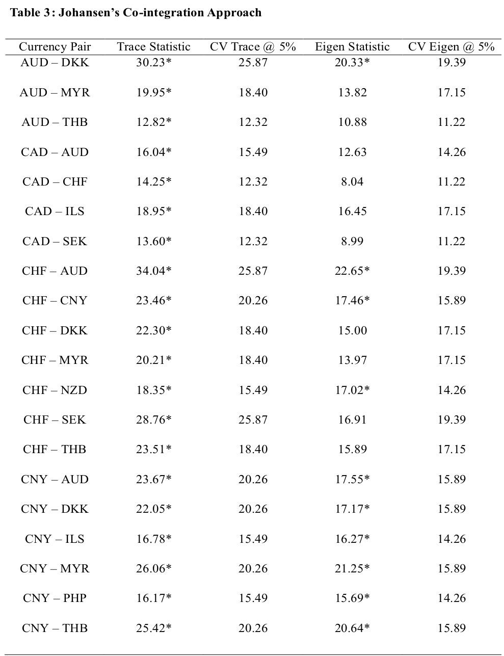
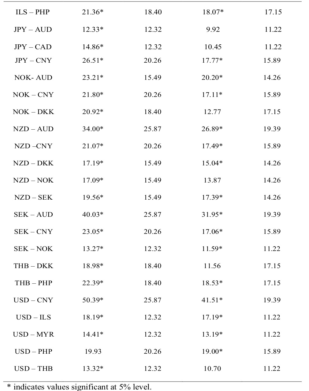
Engle and Granger (1987) proposed that if two time-series are non-stationary and their linear combination is a stationary series, then the two time-series are co-integrated. The co-integrated series move together. The pairs trading strategy works on the idea that currency pairs are co-integrated. We used the Johansen approach (Johansen, 1988) for statistical significance of co-integrating relation between the currency pairs. The Johansen’s approach uses two test statistics namely, the trace statistic or the maximum Eigenvalue for determining the number of cointegrating relations. The trace statistic tests the joint null that the number of co-integrating vectors is less than or equal to ‘r’ (H0: r = r* < k, where r is the rank of the co-integrating matrix, k refers to the number of cointegrating relations) against an alternative that there are more than ‘r’ cointegrating vectors (Ha: r =k). The test proceeds sequentially for r* = 1,2,…k. The first non-rejection of null is the estimate of ‘r’. Similarly, the maximum Eigenvalue tests the null hypothesis that the number of co-integrating vectors is ‘r’ (H0: r =r* < k) against an alternative of ‘r + 1’ (Ha: r = r*+1) cointegration relations. The rejection of null shows the presence of a cointegrating relationship between the currencies. The mathematical representation of the trace test and the eigen value test are given in (4) and (5)

λ_trace= -T ∑_(i=r+1)^n▒〖ln⁡(1-(λ_i ) ̂ 〗) (4) λ_max⁡〖(r,r+1)〗 = -T ln⁡〖(1-λ ̂_(r+1) 〗) (5)

here, (λ_i ) ̂ represents the estimated eigenvalue for the co-integrating matrix.

Estimation of the spread using an error correction model

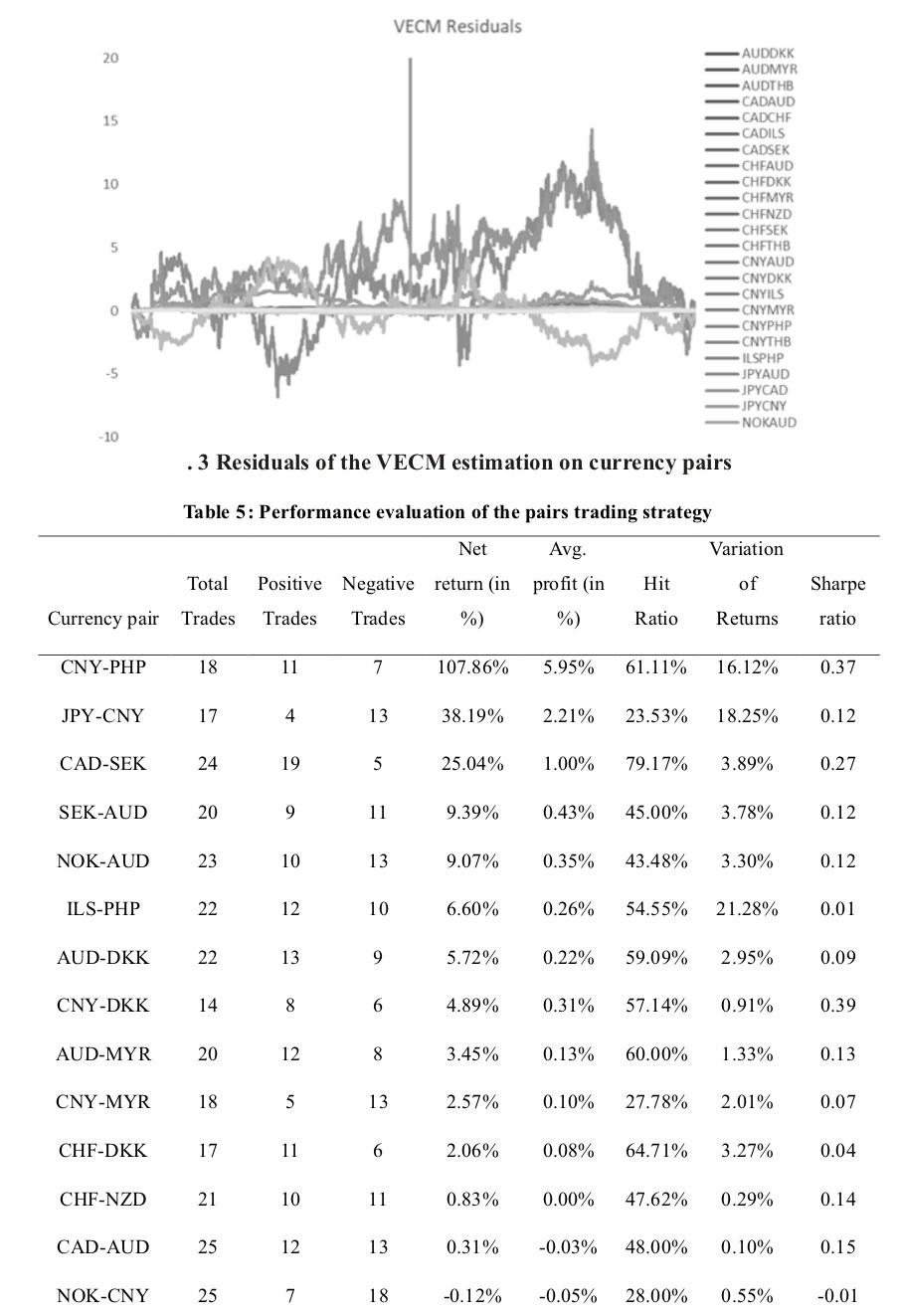
The spread measures the extent of mispricing/discrepancy from the long-term equilibrium relation between the co-integrated currency pairs. The central idea of pairs trading is to follow the contrarian strategy for trading the spread, i.e., an investor enters into a long (short) position in the currencies to trade the spread when the actual value of the spread is larger (smaller) than the predicted threshold value. The contrarian strategy is applied when the spread reverts to an equilibrium value to earn a profit. The spread is uncorrelated with market returns and neutral to market fluctuations (Vidyamurthy, 2004; Elliott, der Hoek, & Malcolm, 2005). In a perfectly market-neutral portfolio, the performance of the long portfolio and the performance of the short portfolio offset each other, and thus an investor is expected to earn roughly the risk-free rate. (Elliott et al., 2005) proposed that the spread should be mean-reverting and stationary. We estimated the spread of the co-integrated currencies using the VECM (Vector Error Correction Model). The residuals of the VECM model should be mean-reverting and stationary for the currency pairs to be cointegrated. The residuals are stationary if their auto-correlation function is zero. If it is not, then taking the first difference of residuals, make them iid (independent and identically distributed), as they followed AR (1) order. The best fit VECM captures the long run relationship of two cointegrated currencies. If X and Y are two non-stationary cointegrated time series with a linear combination represented as (Y_t- γX_t), which is stationary i.e., I (0), then we have,

Y_t- γX_t=(β_(Y_t )-γβ_(X_t ) )+ (ϵ_(Y_t )-γε_(X_t )) (6)

Where, β_(Y_t ),β_(X_t )represent the non-stationary components of Y and X respectively.〖 ϵ〗_(Y_t ), ϵ_(X_t )are errors. The residuals of the VECM should be stationary, The spread is computed as the logarithmic difference between estimated and actual exchange rates between periods t and t+i (wherei =1, 2…n) of long-short currencies. The spread is mean-reverting and stationary if the residuals of the VECM are i.i.d. The mathematical representation of the spreadis given in (7)

ΔS = [log⁡〖(Y_(t+i) )-log⁡(Y_t)]- γ[log⁡(X_(t+i) )-log⁡(X_t)]〗 (7)

The Pairs Trading Strategy

Vidyamurthy(2004)suggested that the co-integrated series should necessarily have an estimated spread which is mean-reverting and stationary. The idea of pairs trading is derived on the premise that there is a long-run equilibrium between the co-integrated pairs; therefore, any deviation from that equilibrium is compensated by subsequent movement in the time series. Bakhach et al., (2018) used a contrarian trading strategy for generating buy and sell signals against the market trend to benefit from the reversal or correction of the short-term mispricing in the exchange rate of currency pairs. Chen and Lin (2017)used a rolling-window approach to estimate the non-parametric one-sided limits for the mean spread and to calibrate the tolerance level or threshold for trading entry and exit signals for securities pairs traded on the US stock exchange. With the above insights, we used a rollingwindow of 250 trading days to estimate the mean spread. A z-statistic is computed to measure the deviation of the spread from the equilibrium (or mean spread). The z-statistics of +2.5 and -2.5 are considered as upper and lower thresholds respectively. The formula of z-statistics for the spreadis given in (8)

z= ((s_i - s ̅))/σ_s (8)

Where ‘si’ represents spread at a time ‘i’ and s ̅ stands for mean estimated spread and σ_s refers to the standard deviation of the spread in the estimation window We applied the contrarian strategy for trading the spread based on the entry and the exit signals. The upper threshold (μ + 2.5Δ) and a lower threshold (μ - 2.5Δ) are computed as +/-2.5 standard deviations away from the meanspread (μ). When the spread has the z-statistic less than -2 or greater than 2, an ‘enter’ signal is generated. When the spread reverts to its equilibrium, the contrarian strategy is applied, and the positions of trade are reversed. At ‘enter’ signal, a portfolio is constituted by taking long-short positions in the currencies. The over-valued currency is sold,and under-valued currency is bought to make the portfolio market-neutral. The positions are reversed at the first ‘exit’ signal following an ‘enter’ signal. Performance evaluation of the pairs trading strategy We performed the back-testing procedure of the pairs trading strategy on the ex-post data. Bakhach, Tsang, and Chinthalapati (2018) used a range of metrics for evaluation of the trading strategy viz., the rate of returns, profit factor, maximum drawdown, win ratio, Sharpe ratio,and the Sortino ratio. In our study, we have used the metrics like – the hit ratio and the Sharpe ratio for evaluation of the strategy along with calculation of average return, net return, return variance and number of positive (negative) trades during the back-testing process. Assume, we generated an ‘enter’ signal for a currency pair, say INR/USD-INR/CNY, having a co-integration ratio of -0.06, and z-score of the spread is 2.8, an investor enters into the long-short position in the INR/USD and INR/CNY currencies respectively. The long-short portfolio is both value-neutral and market neutral. As the currency pair is bought-sold in the proportion of the co-integration ratio (measured by VECM beta), the pair is value neutral. The co-integrated pair is market neutral as it is uncorrelated with market returns. The investor holds on to the portfolio till the ‘exit’ signal is generated when there is mean-reversion of the spread (Z-score should revert to mean 0). The investor reverses the long-short positions in the currencies to earn the arbitrage returns. In the above example, the spread is greater than upper bound at the time ‘t’, sell the currency INR/USD (represented as X) and buy INR/CNY (represented as Y) in the proportion of the co-integration ratio (γ). At ‘exit’ signal at the time, ‘t+i’, sell INR/CNY (Y) and buy INR/USD (X). Figure.1 shows the pairs-trading set up of USD-CNY currency pair. The total return is computed as given in (9), (10) and (11)

S_t= log⁡〖(1+X_t )- γ〗 log⁡〖(1+Y_(t+i))〗 (9) S_(t+i)= log⁡〖(1+Y_(t+i) )- γ〗 log⁡〖(1+X_(t+i))〗 (10) Total Ret= ∑_(i=1)^N▒(〖(S〗_t+ S_(t+i)))/2 (11)

Where N is the total number of trades The average return is computed as the total return divided by the number of trades. Trade is considered as complete if there are no openpositions,i.e., an ‘enter’ trade is squared off with a corresponding ‘exit’ trade. The average return is represented in (12)

Avg.Ret= (Total Ret)/N (12)

The total return and the average return are adjusted for transaction costs as per the rule of the NSE. The transaction cost at the rate of 0.042% (0.04% - exchange charges, 0.002% - clearing charges) is referred from the website Zerodha. The Hit ratio is computed as a ratio of positive trades to a total number of trades for a trading period of a currency pair. It is represented in (13)

Hit ratio= (No. of Positive trades)/( Total number of trades )*100 (13)

The Sharpe ratio (Sharpe, 1994) provides a measure of reward-risk for an investor. It is measured as a ratio of risk-adjusted excess return per unit of risk. It represented below.

Sharpe ratio= (R_p- R_f)/σ_p (14)

WhereRp denotes portfolio returns, Rf is risk-free rate and σ_p denotes the standard deviation of portfolio returns.

Results and Discussion

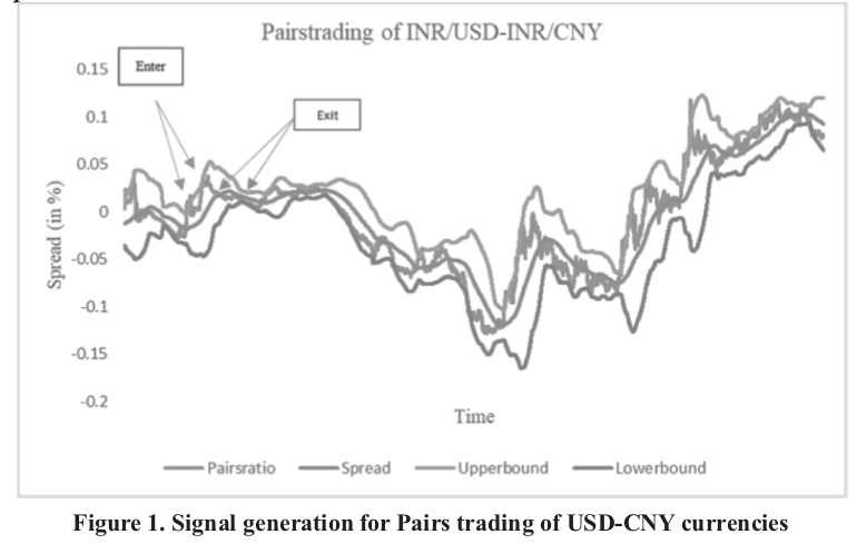
Figure. 2 show the graphical representation of global currencies. The IQR computed as in (1) showed the presence of outliers in three currencies viz., BRL, EUR, and ARS. We have removed these three currencies from further analysis as the rules of statistical arbitrage trading cannot be applied to the extreme observations.

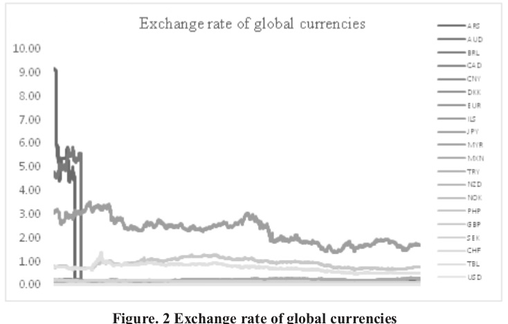
Table 1 shows the correlation between currencies. The correlation coefficient (r)is computed as in (2). We have considered highly correlated currency pairs (r >=0.7 as potential pairs. We found 86 currency pairs with higher correlation. The currencies of major markets like AUD, CAD, CHF, CNY and DKK have a high correlation with all other currencies except PHP, but negative relation with TRY. The GBP has good correlation with the currencies of EU (CHF, DKK, NOK, and SEK), the US (USD, CAD), Australia(AUD), and Asia (only CNY but not with JPY). The Turkish Lira (TRY) has a negative correlation or no correlation at all with other currencies.

Table 1: Correlation analysis of currency pairs

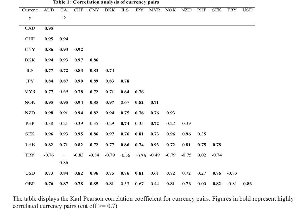
Table 2 shows the results of the AugmentedDickey-Fuller test for non-stationarity of the currencies. The null hypothesis of a unit root for currencies is rejected at 5% level if the ADF statistic is less than the Dickey-Fuller critical value at 5% level of significance. It is observed that the ADF statistic for all currencies is greater than the respective critical values except for EUR. Therefore, the null is rejected only for EUR implying that EUR is stationary at level. All other currencies are non-stationary at level.

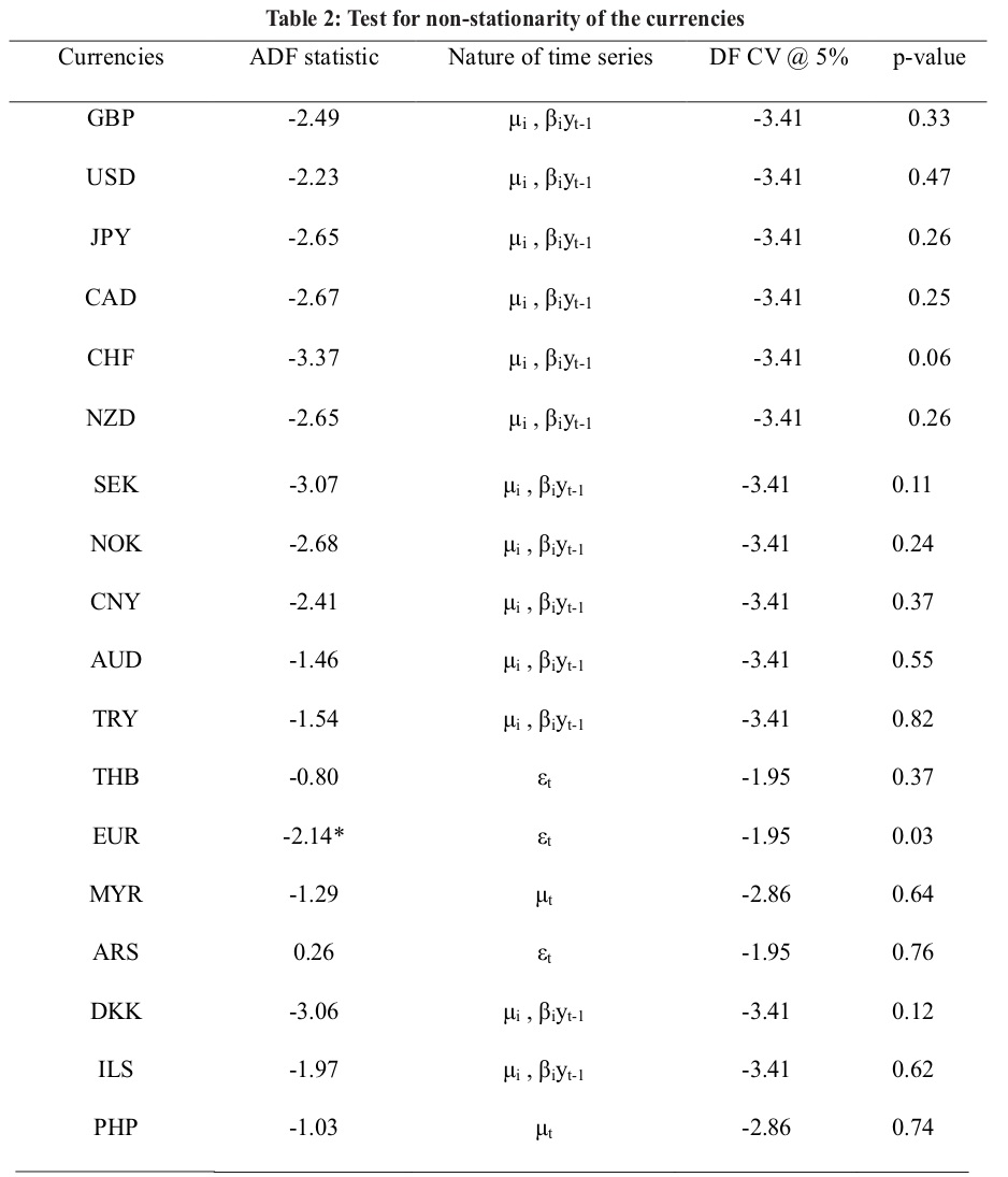
notations are used to describe the nature of the time series,i.e. if it is described by an intercept, a trend or intercept & trend or is yt is purely a function of noise?. The ADF test follows the Dickey-Fuller distribution. The null hypothesis that the time series has a unit root is rejected if the computed ADF statistic is lesser than the critical value of DF distribution. Table 3 provides the result of the trace test and the eigenvalue statistics for testing the number of the co-integrating relationship between the currency pairs. We have referred either the trace statistics or the eigenvalue statistic for determining the co-integrating relationship. In the case of duality in test statistics, we have followed the eigenvalue statistic as the decision criteria for the validation of the null hypothesis that assumes no cointegration relationship of the currencies. The null is rejected for 43 (out of 97)currency pairs indicating at least one co-integrating relation between the currencies. Table 4 shows the estimates of the best fit VECM for the cointegrated currency pairs. We performed the OLS regression of the currency pairs. As the OLS regression is spurious, fitting an error correction model measures the non-spurious relationship between the currencies. We fitted the best fit VECM model with an appropriate lag length chosen based on the SIC penalty criteria. We performed VECM estimation and reported the parameters viz., the intercept and the VECM beta (cointegrating coefficient).The difference between the actual exchange rate and the estimated exchange rate gives the VECM residuals. We performed the residual diagnostics,i.e. the ADF test for stationarity on the residuals and found that the null hypothesis is rejected for three currency pairs viz.,CAD-ILS, CHF-DKK, CHF-THB implying that residuals are mean-reverting and stationary. The residuals of the other currency pairs followed AR(1) order and became stationary after first difference. Figure.3 shows the graphical representation of the VECM residuals for all currency pairs. Table 5 shows the results of the back-testing of the pairs trading strategy. The table shows the performance evaluation measures like the net return, average profit, the hit ratio and the Sharpe ratio computed as in (11), (12), (13) and (14) respectively. Table 6 describes the currency pairs for the performance evaluation of the strategy. It is found that CNY-PHP yielded a maximum average profit of 5.95% with a hit ratio of 61% and the Sharpe ratio of 0.3 indicating lower returns for given risk. The variation in expected trading returns is so huge i.e. 16.12%. A Sharpe ratio of 0.6 is assumed to be preferable as a return-risk profile for currency trader. CAD-SEK has the highest hit ratio of 79%. The risk-return profile is low for CAD-SEK as it has an average return of 1% with a deviation of 3.89% and the Sharpe ratio is 0.27. CNY-DKK has the highest Sharpe ratio of 0.39 with a hit ratio of 57% and the average profit of 0.31% (return variance of 0.91%). CNY-DKK may givemaximum returns for a given risk level. There are 26 currency pairs (out of 39) with negative Sharpe ratios, implying non-profitable currency pairs for arbitrage trading viz., NOK-CNY, CAD-CHF, CHF-AUD, CNY-ILS, NOK-DKK, NZD-AUD, USD-MYR, NZD-CNY, CHF-MYR, NZD-SEK, USD-CNY, SEK-CNY, CNY-THB, NZD-NOK, USD-ILS, CHF-SEK, USD-PHP, AUD-THB, CAD-ILS, NZD-DKK, CNY-AUD, THB-PHP, CHF-THB, JPY-CAD, JPY-AUD and USD-THB. It is observed from Table 6 that there are 11 and 13 currency pairs with positive average profit and net trade returns, respectively, after adjusting for transaction costs. The 11 currency pairs include CNY-PHP, CNY-JPY, CNY-MYR, CNY-DKK, AUD-SEK, ADU-NOK, AUD-DKK, AUD-MYR, CAD-SEK, CHF-DKK and ILS-PHP. Three currency pairs viz., CNY-PHP, CAD-SEK and AUD-MYR have yielded positive average profit, positive net trade returns with a hit ratio of above 60%, indicating a good record of back-testing results. However, the Sharpe ratios are less than 0.3 (30%) indicating higher risks taken and lower returns earned.

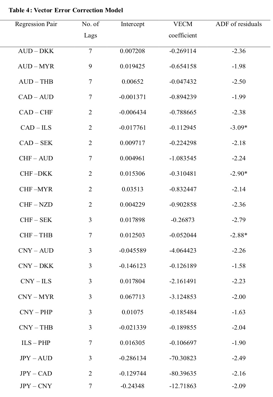
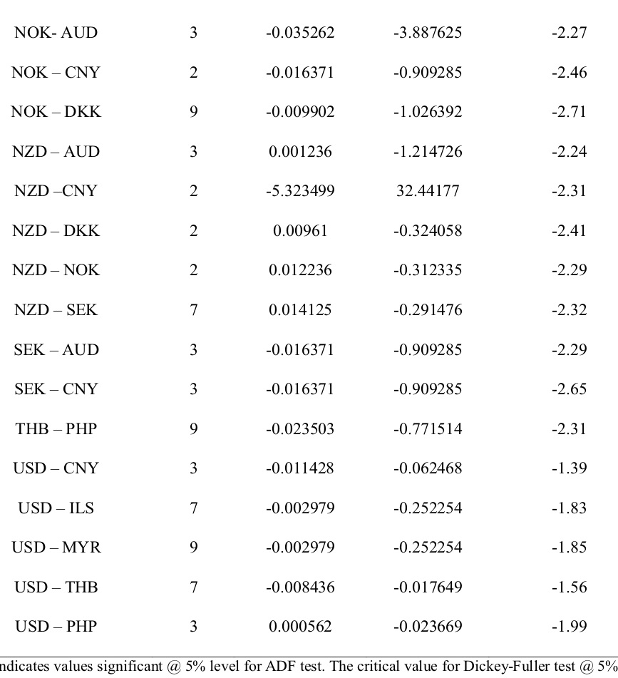
is -2.86. Column 1 (Regression Pair) identify the cointegrated currency pairs. We performed the OLS regression on the pair and found that fitting an error correction model makes the regression non-spurious. Column 2 indicates the appropriate lag length used in the VECM estimation, selected based on the SIC penalty criteria. The lag with the lowest penalty criteria is the appropriate lag length. Column 3 shows the estimated intercept value from the VECM estimation. Column 4 shows the estimated VECM beta. Column 5 indicates residual diagnostics statistics. We performed the ADF test on the VECM residuals for stationarity. The VECM residuals not stationary at level followed the AR (1) order.

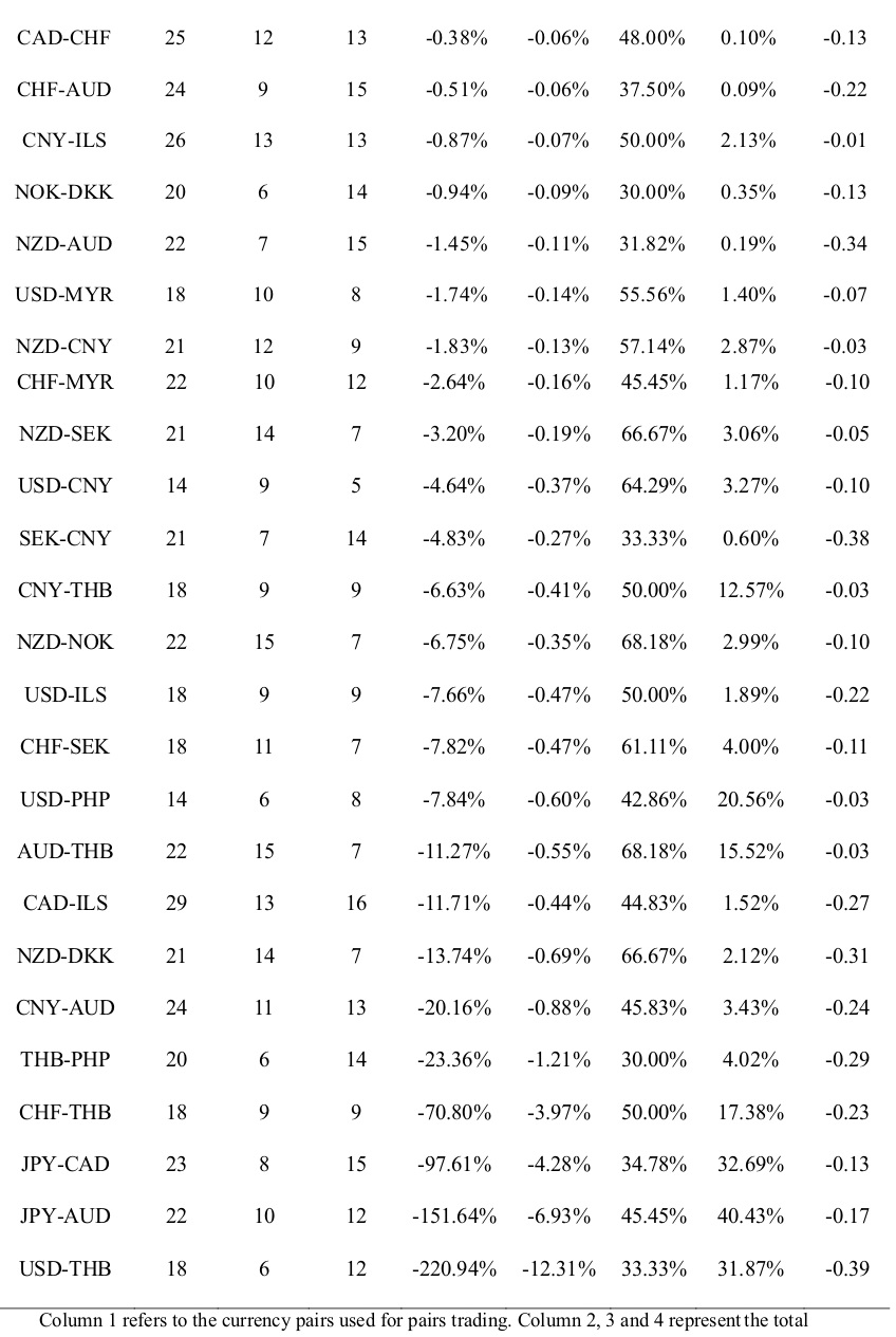
Column 1 refers to the currency pairs used for pairs trading. Column 2, 3 and 4 represent the total number of trades carried out, no. of positive trades and no. of trades with negative returns, respectively, for each currency pair. Column 5 and 6 represent total return and average profit computed as in (11) and (12) respectively. The total return and the average profit are adjusted for the transaction cost available for trading on the NSE @ 00.42%. Column 7 represents the ratio of positive trades to total trades for each currency pairs,i.e. Hit ratio computed as in (13). Column 8 represents the reward-risk ratio for trading in the currency,i.e. the Sharpe ratio computed as in (14). The ‘risk-free’ rate is assumed to be 0 for calculations purpose.

Findings and Conclusion

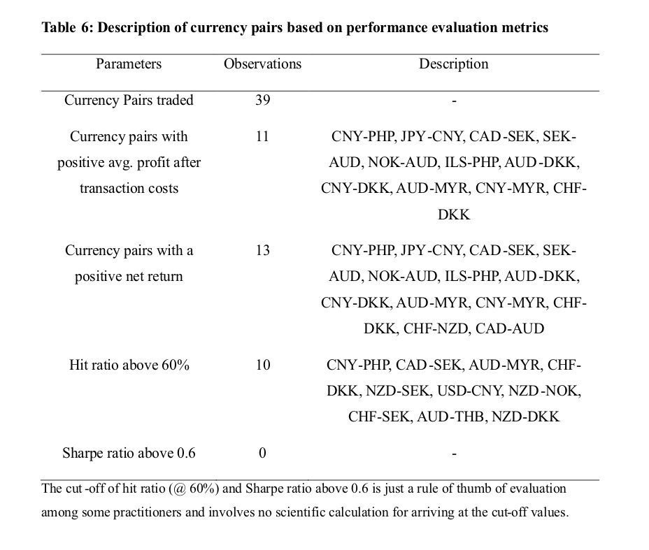
The global integration of economies has led to the co-movement of currencies of the nations. If markets were to be efficient in the weak-form, trading and speculation in currencies should not have yielded to abnormal returns without taking an additional risk. We studied the statistical arbitrage trading process under the pairs trading framework on 20 global currencies. We found 39 currency pairs as potential currency pairs for trading as they shared at least one cointegrating relationship. The back-testing results showed that 13 currency pairs (out of 39) yielded positive net trading returns and 11 currency pairs (28%) generated the positive average profit. The negative Sharpe ratios for 26 currency pairs indicated that they are un-profitable pairs. Three currency pairs viz., CNY-PHP, CAD-SEK and AUD-MYR earned the positive average profit and net trading returns with a hit ratio of above 60% indicating a good back-testing performance. The lower Sharpe ratios (<0.3) indicate lower risk-return profile for the currency arbitragers. Our results supported that findings of Bakhach, Tsang, and Chinthalapati (2017, 2018) and (Galeshchuk, 2017; Galeshchuk & Mukherjee, 2017) that currency pairs trading is profitable. They identified EUR-CHF, GBP-CHF, EUR-USD, GBP-USD, and USD-JPY as profitable pairs. Alternatively, our study showed CNY-PHP, CAD-SEK and AUD-MYR as profitable currency pairs. The study explored potential currency combinations of emerging Asian economies viz., Myanmar (MYR), Philippines (PHP), China (CNY) with Canada (CAD), and Australia (AUD) for rule-based arbitrage trading. We usedcorrelation and cointegration analysis for identification of pairs, VECM model for estimation of the spread on the ex-post data. The findings of the study are no way conclusive evidence that the currency pairs identified are robust. The results may vary if a different estimation model or the out-sample estimation is used. More studies robust to estimation methods, parameters optimisation in back-testing process are needed in order to explore tradable pairs across diverse asset classes given the challenges of limited arbitrage opportunities, illiquidity of currency contracts due to huge contract value and volume, market microstructure constraints, extreme volatility, and the regulatory constraints for pairs trading.

References:

Auld, T., & Linton, O. B. (2019). The behaviour of betting and currency markets on the night of the EU referendum. International Journal Of Forecasting, 35(1), 371–389. https://doi.org/10.1016/j.ijforecast.2018.07.014
Avellaneda, M., & Lee, J. H. (2010). Statistical arbitrage in the US equities market. Quantitative Finance, 10(7), 761–782. https://doi.org/10.1080/14697680903124632
Bakhach, A. M., Tsang, E. P. K., & Raju Chinthalapati, V. L. (2018). TSFDC: A trading strategy based on forecasting directional change. Intelligent Systems in Accounting, Finance and Management, 25(3), 105–123. https://doi.org/10.1002/isaf.1425
Bakhach, A., Tsang, E., Ng, W. L., & Chinthalapati, V. L. R. (2017). Backlash Agent: A trading strategy based on Directional Change. In 2016 IEEE Symposium Series on Computational Intelligence, SSCI 2016. https://doi.org/10.1109/SSCI.2016.7850004
Chaboud, A. P., Chernenko, S. V., & Wright, J. H. (2008). Trading activity and macroeconomic announcements in high-frequency exchange rate data. Journal of the European Economic Association, 6(2–3), 589–596. https://doi.org/10.1162/JEEA.2008.6.2-3.589
Chen, C. W. S., & Lin, T. Y. (2017). Nonparametric tolerance limits for pair trading. Finance Research Letters, 21, 1–9. https://doi.org/10.1016/j.frl.2016.11.002
Choi, M. S. (2011). Momentary exchange rate locked in a triangular mechanism of international currency. Applied Economics, 43(16), 2079–2087. https://doi.org/10.1080/00036840903035969
Dickey, D. A., & Fuller, W. A. (1979). Distribution of the Estimators for Autoregressive Time Series with a Unit Root. Journal of the American Statistical Association. https://doi.org/10.2307/2286348
Elliott, R. J., der Hoek, J., & Malcolm, W. P. (2005). Pairs trading. QuantitativeFinance, 5(3), 271–276. https://doi.org/10.1201/b18325
Engle, R. F., & Granger, C. W. J. (1987). Co-Integration and Error Correction : Representation, Estimation, and Testing, Econometrica, 55(2), 251–276. https://doi.org/10.2307/1913236
Fama, E. F. (1984). Forward and spot exchange rates. Journal of Monetary Economics. https://doi.org/10.1016/0304-3932(84)90046-1
Frenkel, J. A., & Levich, R. M. (1977). Transaction Costs and Interest Arbitrage : Tranquil versus Turbulent Periods. Journal of Political Economy. https://doi.org/10.1086/260633
Galeshchuk, S. (2017). Technological bias at the exchange rate market. Intelligent Systems in Accounting, Finance and Management, 24(2–3), 80–86. https://doi.org/10.1002/isaf.1408
Galeshchuk, S., & Mukherjee, S. (2017). Deep networks for predicting the direction of change in foreign exchange rates. Intelligent Systems in Accounting, Finance and Management, 24(4), 100–110. https://doi.org/10.1002/isaf.1404
Gatev, E., Goetzmann, W. N., & Rouwenhorst, K. G. (2006). Pairs trading: Performance of a relative-value arbitrage rule. Review of Financial Studies, 19(3), 797–827. https://doi.org/10.1093/rfs/hhj020
Hansen, L. P., & Hodrick, R. J. (1980). Forward Exchange Rates as Optimal Predictors of Future Spot Rates: An Econometric Analysis. Journal of Political Economy. https://doi.org/10.1086/260910
Jacobs, H., & Weber, M. (2015). On the determinants of pairs trading profitability. Journal of Financial Markets, 23, 75–97. https://doi.org/10.1016/j.finmar.2014.12.001
Johansen, S. (1988). Statistical analysis of cointegration vectors. Journal of Economic Dynamics and Control. https://doi.org/10.1016/0165-1889(88)90041-3
Krauss, C. (2017). Statistical Arbitrage Pairs Trading Strategies: Review And Outlook.Journal of Economic Surveys. https://doi.org/10.1111/joes.12153
Neely, C. J., & Weller, P. A. (2013). Lessons from the evolution of foreign exchange trading strategies. Journal of Banking & Finance, 37(10), 3783–3798. https://doi.org/10.1016/j.jbankfin.2013.05.029
Perlin, M. S. (2009). Evaluation of pairs-trading strategy at the Brazilian financial market. Journal of Derivatives and Hedge Funds. https://doi.org/10.1057/jdhf.2009.4
Röthig, A. (2012). Cross-speculation in currency futures markets. International Journal of Finance and Economics. https://doi.org/10.1002/ijfe.462
Sharpe, W. F. (1994). The Sharpe Ratio. The Journal of Portfolio Management. https://doi.org/10.3905/jpm.1994.409501
Shleifer, A., & Vishny, R. W. (1997). The Limits of Arbitrage. The Journal of Finance. https://doi.org/10.1111/j.1540-6261.1997.tb03807.x
Vidyamurthy, G. (2004). Pairs Trading: Quantitative Methods and Analysis. John Wiley&Sons Inc.