Editorial Board

A Refereed Monthly International Journal of Management

Different VAR for Developing and Developed Nations because of Market Efficiency

Author

Dr. Shailesh Rastogi Professor (Finance) Symbiosis Institute of Business Management (Pune) Gram: lavale; Tal: Mulshi (Pune, India) krishnasgdas@gmail.com

Ashok Patil Assistant Professor Kirloskar Institute of Advanced Management Studies

Akanksha Goel Research Scholar Symbiosis International (Deemed University)

Abstract

The aim of this paper is to compare the performance of VaR among Nations. This paper employs the method proposed by Diebold, Schuermann, and Stroughair (1998) and McNeil and Frey (2000) in order to filter the return data to obtain i.i.d residuals by fitting ARMA-GARCH models.The model that shows the lowest percentage failure rate in VaR in out-of-sample period is identified as the best GARCH model to estimate VaR. The conditional and unconditional coverage tests are conducted to assess the adequacy of VaR estimates.Persistent I-GARCH-t models give the best VaR estimates in developing nations while asymmetric e-GARCH-t models yield the best VaR estimates for developed nations.

Keywords– Variances, Value at Risk, Market Risk, Indices, GARCH Models

Introduction

Different VAR for Developing and Developed Nations because of Market Efficiency

Riskis defined as an uncertainty which may lead to losses (Holton, 2004). The risk in business can be divided into two broad categories: systematic and unsystematic risks. Unsystematic risks are easy to be estimated, but systematic risks are difficult to be estimated (Beja, 1972; Nandha and Hammoudetr, 2007). There are various methods which are applied to estimate the systematic risks, e.g., standard deviation, beta. Value at Risk (VaR) is one such method to estimate systematic risk or to be precise, to estimate market risk. VaR can be used for estimating market risk present in individual assets, portfolio, or in any other security (Linsmeier and Pearson, 2000). VaR, over the period, became a favorite tool to measure market risk, even for banks (Berkowitz and O’brien, 2002; Dimson and Marsh 1995, Aloui and Hamid 2015; Chong, 2004). Earlier, Basel Accord [1]was heavily criticized for not addressing market risk in its fold. However, in 2009, after much deliberation, VaR became part of Basel II norms to measure the market risk. Along with popularity, VaR was also widely critiqued. The most prominent criticism which VaR faces is on the methodology part to estimate VaR (Bekiros and Georgoutsos, 2005; Hung, Lee and Liu, 2008). Methods of VaR measurement can be divided into two broad categories: parametric and non-parametric methods. Brook and Persand (2002) endorse this division and classify all the methods of estimating VaR into these two categories. Parametric methods (Variance-covariance, GARCH based methods,etc.) use return distribution to calculate VaR whereas non-parametric methods (Historical simulation, Extreme value theory,etc.) do not involve return distribution. There are many studies published that explore the best method to capture VaR. There are many comparisons made between parametric and non-parametric methods. Most of them are in favor of parametric methods (Engle and Manganelli, 2001; Ghorbel and Souilmi, 2014; Vlaar, 2000). Also, there are numerous studieswhich have profusely compared various parametric models and found that GARCH models are placed above non-GARCH models for the estimation of VaR (Orhan and Koksal 2012). In addition to this,several studies compare historical volatility and implied volatility methods to estimate VaR (Bams, Blanchard and Lehnert, 2017). Literature is also replete with comparing different GARCH models (within parametric models) to estimate VaR, but there is no unanimity for the best GARCH method. The other studies also share the similar results (Aloui and Hamida, 2015; Mabrouk and Aloui, 2010; Degiannakis, Floros and Dent, 2013; Obi, Sil and Choi, 2010; Shao, Lian, and Yin, 2009). Presecsu and Stancu (2011) argue that plain-vanilla GARCH (1,1) model is superior to other GARCH models. So and Yu (2006) also find evidence for IGARCH (Integrated GARCH Models) and FIGARCH (Fractionally Integrated GARCH) models to be better than other GARCH models. Among GARCH-based parametric models (to estimate VaR), it was observed that different studies support different GARCH models. All the studies have been done on different indices (of different nations) and at different time periods. Stock indices in different nations have a different level of market efficiency and maturity. This difference may be more severe between developed and developing economies (Aitken and Siow, 2003; Chan, Gupand Pan, 1997). Due to this reason, stock-indices of different nations may require different GARCH models to estimate VaR. This observation is the research problem of this paper. This study addresses the problem of explaining the variation in the choice of a GARCH model to estimate VaR. Thus, the current study has the following objectives:

1.	To explore the reason(s) for variation in the selection of different GARCH models to estimate VaR among Nations/indices. 
2.	To identify better GARCH models to estimate VaR
3.	To compare GARCH models between developing and developed nations to estimate VaR

This paper has been divided into seven sections. The next section is on review of literature. The third section presents the theoretical framework of the paper. The fourth section elaboratesthe data and methodology. The fifth section shares the empirical results of the study. The sixth section of the paper discusses the results of the paper followed by conclusion and policy implication in the last section.

2. Review of literature

Literature review in this paper has been divided into four categories. The first category is for the acceptability and popularity of VaR as a tool to measure market risk. The second category provides the evidence of criticism of VaR. The third category is on the evidence of the theory that Nations require different GARCH models to estimate VaR. Fourth and the last category is on the evidence of the requirement of different GARCH models to estimate VaR for developing and developed nations.

2.1 Popularity of VaR

The financial turmoil of 1987 was a turning point in the history of stock markets across the world. The turning point gave a considerable flip to the clamors for a new tool to measure market risk more effectively. Academia, researchers, and industry all felt the need for a new tool to measure market risk which would be feasible, easy to calculate and acceptable. Eventually, in 1994, JP Morgon formally proposed Value at Risk (VaR) as a market risk measurement tool to fill the gap. Since then, VaR has been available to the world for its use, and its popularity has had no bound.VaR as a market risk measurement tool is quite popular not only in the stock market but also in the exchange rate market (Brooks and Persand, 2003; Angelovska, 2013). Lechner and Ovaert (2010) posit that VaR isan accessible and acceptable risk management tool among its contemporaries. Linsmeier and Pearson (1996) and Dowd (2007) highlight a few characteristics behind the popularity of VaR as a market risk measurement tool. First, it is a common and a consistent measure of risk across all the asset classes of investments. Second, it takes different risk factors into consideration even if they cancel each other. Sharma, Sharma,and Alade (2004) also document different reasons for VaR’s popularity: 1) acceptance of VaR due to Basel Accord; 2) integration of the markets in the world where VaR fits in better than other models; and 3)advancements in Information and communication technology (ICT).

2.2 Criticism of VaR

VaR has its share of criticism as well. VaR was criticized by Hoppe (1999) and Taleb & Jorion (1997) because VaR involves complex mathematics and statistics. Long-term capital market’s (LTCM) downfall was highlighted as an example of the failure of VaR in measuring market risk in time (Dungey et al., 2006). Ghorbel & Souilmi (2014) and Vlaar (2000) strongly support parametric models of estimating VaR as compared to non-parametric methods. Even within parametric methods, Variance-covariance approach (VCV), which was much popular during those days, did not stand the test of time. As volatility clustering and asymmetry were discovered in stock market time-series, VCV lost its relevance (Karmakar, 2007). McMillan and Kambouroudis (2009) find evidence that GARCH performs better than Risk Metric method to estimate VaR (Risk Metric method was the original method to estimate VaR as JP Morgan used this method in 1990).

2.3 Different nation, different GARCH to estimate VAR

No study exhibits results unilaterally in favor of one type of GARCH models to estimate VaR. Predescu and Stancu (2011) explain that symmetric-GARCH models perform better than non-symmetric models. They used a portfolio of US, UK and Romanian stock exchanges in their study. So and Yu (2006) support long-memory and persistent-GARCH models and do not support the plain-vanilla GARCH model. So and Yu use 12 world market indices to find their result. Orhan and Koksal (2012) show result in favor of the plain-vanilla GARCH (1,1) model and t-distribution as compared to other GARCH models. Orhan and Koksal (2012)t use stock-indices of Brazil, Turkey, US, and Germany. Maghyereh and Al-zoubi (2006) show that for the Middle-east and African nations conventional VaR estimation methods give faulty results.

Hypothesis 1: Suitability of GARCH model to estimate VaR is dependent upon nation/index

2.4 Developed vs. Developing nations and GARCH to estimate VaR

Aitken and Siow (2003) and Chan, Gup and Pan (1997) highlight a new line of thinking. They exhibit that the use of the GARCH model is dependent upon stock market efficiency and its maturity. This logic highlights that developing nations and developed nations will naturally have different choices for GARCH model to estimate VaR. Orhan and Koksal (2012) take two nations from each basket of developing and developed nations to estimate VaR by GARCH models. However, they did not address the issue of comparing performances of developed versus developing nation to estimate VaR. Most of the existing studies on comparing GARCH models for estimating VaR are done on the indices of developed nations (Aloui and Hamida, 2015; Angelovska, 2013; Maghyereh and Awartani, 2012). The issue of comparison between developed and developing nations have not been addressed much in the literature referred by the author. Hypothesis 2: Developing and developed nations require different GARCH models to estimate VaR.

3. Theoretical framework

The role of the GARCH model in estimating VaR is limited to the estimation of variance, which is an important input variable. This paper uses GARCH based parametric methods to estimate VaR as proposed by Dowd (1998). The method used by Dowd to estimate VaR is also used by So and Yu (2006) and Predescu and Stancu (2011) in their respective studies

Using equation 4, VaR can be estimated at anyone of the confidence levels (or at any level of significance or probability levels). In the present paper, we have taken two confidence levels: 1% and 5%. Correspondingly, the value of z can be taken for both the confidence levels, as discussed below.

Confidence Levels (α)	Zα/2
1%	2.326
2.5%	1.960
5 %	1.645

Other than prices of indices in the equation 4, there are two input variables: the z values corresponding to each confidence level and standard deviation. The current paper takes reference from So and Yu (2006) to use Equation 4 to estimate VaR. As discussed in the next section (Section 4.2), nine GARCH-based methods have been used in the current paper to estimate standard deviation. Using all the nine methods, we get nine different VaR estimate for each index

4. Data and methodology

4.1 Data

Data for this paper has been collected through the following websites of Yahoo (www.in.finance.yahoo.com) and Investing (www.in.investing.com). Return series have been calculated by taking the natural log of the price series. The daily closing prices have been taken from January 2010 to November 2015. The period of financial crisis of 2007 has been intentionally excluded in the period of study. Chong (2004) evinces that the behavior of stock prices during normal and abnormal periods are not the same. Due to this reason, we have not taken the irregularperiod of financial crisis in 2007 to avoid the abnormal periods.

4.1.1 Selection of stock indices

As we want to cater to as many as possible stock exchanges in our study, we taketen stock indices in this paper. Literature supports ten stock exchanges as an appropriate number of stock indices for comparison of GARCH models (So and Yu, 2006; Presescu and Stancu, 2011; Orhan and Koksal, 2012). Further, to compare the performance of developing and developed nations, we take five stock indices from each group. Literature is replete with the examples of developing and developed nations. The same references are appliedto the selection of developing and developed nations in this paper (Nielsen, 2011; World Economic Situation and Prospects, 2016). BRICS in itself is a representative of developing nations (Wilson and Purushothaman, 2003; O’Niel and Poddar, 2008). Therefore, all the five nations of BRICS have been considered for representing developing nations in this paper. Following five developed nations are shortlisted in this paper for further analysis by using market efficiency as a criterion:the USA, the UK, Japan, Canada and South Korea (Mensi, 2012; Phan and Zhou 2014; Aitken and Siow, 2003; Lim 2007) (Table 1). Stock exchanges in different nations work on different timelines. Therefore, data cleaning is essential. After data cleaning and bringing parity on dates, 1442 observations are finally considered for further analysis. All the return series are stationary at the level which is appropriate for further analysis. Among the ten indices, RTSI (Russia) and IBOVESPA (Brazil) give negative mean-return. Lowest return i.e. maximum loss is for Nikkei (Japan) and South Africa in developing nations. The maximum return is for South Africa whereas it is Nikkei (Japan). Volatility measured by daily standard deviation is the least for Canada and lowest for BSE Sensex (India) in developing nations. All the ten indices have negative skewness,and RTSI has the highestkurtosis overall and Nikkei (Japan) in developed countries. None of the return series is normally distributed although presence of ARCH effect and dependence is observed. (Table 2).

4.2 Methodology

4.2.1 Selection of GARCH Models

Nine types of GARCH models have been selected for the comparative analysis of the performance of VaR. Stock indices have the following properties which differentiate them from the other type of time series: fat tails (leptokurtic), leverage effect or asymmetry, volatility clustering, non-normalcy in the error distribution and long memory in the variances. Different GARCH models overcome these short-comings differently. In-spite-of the considerable acceptance of GARCH-methods to estimate VaR, unanimity for one particular type of GARCH model, is never realized. GARCH family of models can be clubbed into five clusters: long-memory models, asymmetric models, persistent models, volatility clustering models and fat-tailed models (Degiannakis, 2004; Kasman 2009). Moreover, each GARCH model can further be divided by the density function of error distribution: Normal distribution (Gaussian distribution) and Non-normal distribution (Student’s-distribution). The proposed nine models are EWMA (Exponential Weighted Moving Average), GARCH (1,1), IGARCH, CGARCH, EGARCH. The latter four models are further divided into two on the basis of density function of error distribution as discussed in the above paragraph. Therefore, altogether nine GARCH models are used for the analysis. The natural candidate for non-parametric VaR modeling is EVT (Extreme Value Theorem), however it is inappropriate in the light of the i.i.d. assumption of the returns data. Alternatively, one may apply an EVT on an appropriately filtered data using GARCH models that yield i.i.d. residuals. Diebold, Schuermann, and Stroughair (1998) propose such a method for fitting time-varying model on the data and then estimating i.i.d. residuals enabling to apply EVT on these residuals. A specialized case of above method is tested by McNeil and Frey (2000) by filtering the data using Gaussian AR (1)-GARCH (1, 1). This paper first identifies the suitable ARMA model based on the lowest AIC criterion and then fits the GARCH (1,1) model to the returns data, to test if residuals are i.i.d. If the residuals are i.i.d., the model output is used for further analysis. The two-step process employed in this paper is as follows:

•	Estimate an appropriate ARMA-GARCH model so as to have i.i.d. residuals
•	Apply EVT theory to the residuals obtained as above in order to derive VaR estimates

4.2.2 Data Analysis Methods

Log returns are tested for the presence of autocorrelation by visualizing the ACF, PACF plots and are tested for independence using Ljung-Box Q-statistic. If autocorrelation and/or dependence in the series is found, a suitable ARMA model is identified to make the series serially uncorrelated. The presence of autocorrelation is visualized by ACF and PACF plots. The independence is tested by using Ljung-Box Q-statistic. The presence of ARCH effect is tested using Engle’s ARCH test. If ARCH effect is present in the series, a suitable GARCH model is identified. The data is filtered with an appropriate ARMA and Risk Metrics, GARCH, e-GARCH, c-GARCH, I-GARCH models under the assumption of Gaussian normal, and Student t-distribution of residuals. (Readers are referred to Kuester, Mitinik and Paolella (2006) for comprehensive reading on the comparison of alternative strategies in predicating VaR.). The standardized residuals and squared standardized residuals of the above AR (1)-GARCH (1, 1) models are tested for independence using weighted Ljung-Box test and ARCH-LM test to test whether ARCH effect is present in the residuals. Further, the fitted models are used to forecast 1-day ahead forecast for 300 out-of-sample observations and to derive estimates of VaR at different confidence levels of 1%, 2.5% and 5%. The estimates of VaR generated as above are backtested for its adequacy using Kupiec (1995) for unconditional coverage and Christoffersen (1998) for unconditional coverage. The GARCH model that passes both the unconditional and coverage tests and have the lowest failure rate in VaR is identified as the best model for the given data series (Zikovic, 2007).

5. Empirical results

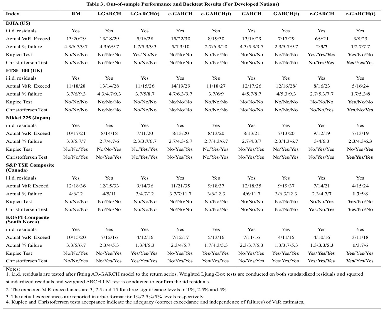
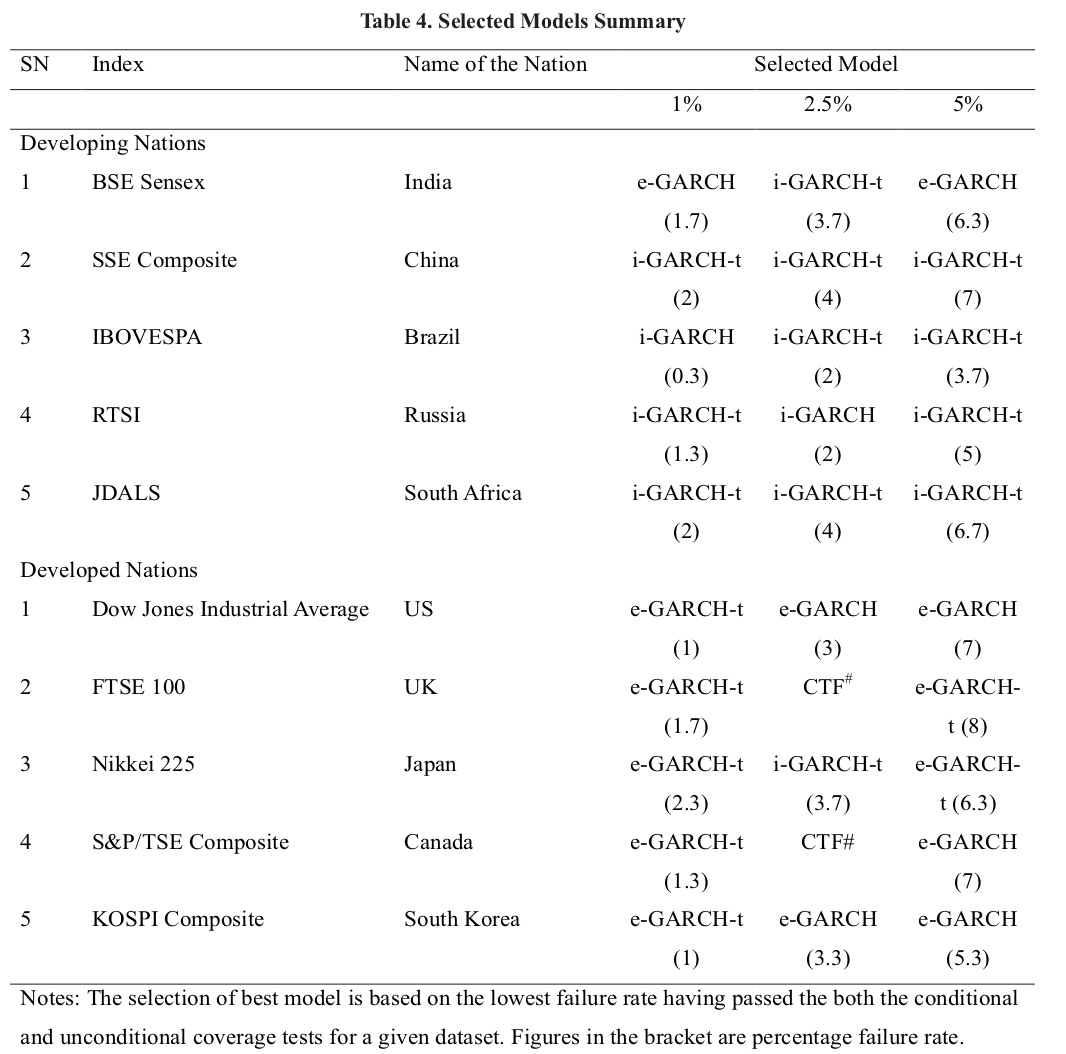
Log returns series of all the developing and developed nation in this study have negative skews and positive kurtosis indicating that all the series have large negative returns occurring more often. The normality tests confirm that none of the series are normally distributed. Test results on all the ten return series in this study found that log returns are not auto-correlated and are independent. On the other hand, the squared return series are serially correlated and ARCH effect is indicated by the tests. Therefore, GARCH models, both symmetric and asymmetric are fit on the return series to remove the presence of heteroscedasticity (Zikovic, 2007). This study employs conditional EVT, also called GARCH-EVT developed by Diebold, Schuermann, and Stroughair (1998) and McNeil and Frey (2000). In the first step, GARCH models are employed to obtain independent and identically distributed residuals and in the second step standardized residuals are fitted using EVT framework. This method combines the time-varying volatility identified by GARCH models with the extreme value performance. As outlined in the methodology section, GARCH models are fit to the log-return series and its residuals are found to be i.i.d. validating the requirement before the EVT is applied on the data. Dynamic Backtesting:After validating the GARCH models, daily VaR are estimated based on 300 one-day ahead forecasts at 95%, 97.5% and 99% confidence level. All the three levels are used for out-of-sample backtesting of VaR in line with the Basel II Backtesting requirements. Out-of-sample backtesting: A one-day ahead VaR estimates are made at 95%, 97.5% and 99% confidence level based on a rolling window forecasts for a given country. The exceedance ratio of the actual number of violations (exceedances) and total number of observations is used to assess the performance of each model. The performance of the models is tested using unconditional coverage test (Kupiec 1995) and conditional coverage (Christoffersen, 1998) tests and are summarized in Table 2 for 1%, 2.5% and 5% confidence levels for developing countries and in Table 3 for developed countries. The null hypothesis under Kupiec test requires that expected exceedances are equal to actual exceedances. The null hypothesis under Christoffersen test requires additional condition of independence of failures (exceedances) over the time period i.e. the actual exceedances are not only equal to the expected exceedances but also are independent of each other. In order to validate the model, the test should not reject the null hypothesis in both the tests. Results of the analysis are reported in three steps. The firststep is on the comparative analysis of GARCH models for estimating VaR. In this step, the emphasis is upon the performance of GARCH models to estimate VaR across ten nations and three confidence levels. The least percentage failure rate is for I-GARCH model (0.3) whereas maximum percentage failure rate is of RM model (12). As discussed earlier, the lesser the percent failure rate, the better the performance. The results mentioned in Table 2 and Table 3 and summarized Table 4imply that RM, c-GARCH, c-GARCH-t, GARCH, GARCH-t had inferior results than the remaining four models (I-GARCH, i-GRACH-t, e-GARCH, e-GARCH-t) in estimating VaR. Results from Table 2 indicate that for BSE Sensex (India) data two models e-GARCH and I-GARCH pass the necessary tests but e-GARCH performs better at 1% and 5%. For SSE Composite (China) only I-GARCH-t passes both the tests. All models pass the coverage tests for IBOVESPA (Brazil) but the best model is I-GARCH-t. RTSI (Russia) index is best captured through I-GARCH-t although all other models pass the coverage tests. For JDALS, I-GARCH-t model performs the best after passing both the coverage tests. Overall, for developing countries I-GARCH-t model gives the best results. Results from Table 3 indicate that for US data, the best models that describe the VaR correctly are e-GARCH and e-GARCH-t. No models other than e-GARCH-t gives better results for FTSE 100 (UK) data at 1% and 5%. For Nikkei 225 data, e-GARCH-t model give better results for 1% and 5% whereas it is I-GARCH-t at 2.5% level. TSE Composite index (Canada) show better results under e-GARCH and e-GARCH-t models for 1% and 5% levels respectively. In the case of South Korea the best results are reported by e-GARCH-t for 1% level and e-GARCH for 2.5% and 5% level. Overall, the better results are provided by e-GARCH-t models. The second step of the result is based upon the performance of VaR for of all the three confidence levels. It has been reported that 1% probability levels give better results than the other two confidence levels. In case of developing nations’ case, the minimum and maximum values of the percentage failure at 1% are 0.3 and 2, respectively. The similar minimum and maximum values of the percentage failure at 2.5% confidence levels are 2 and 4 respectively. At 5% confidence level, minimum and maximum values of the percentage failure are 3.7 and 7 respectively. This highlights that the results for VaR at 1% confidence level are better than the performance at 2.5% and 5%. The same results have been found for developed nations as well and for all the nine GARCH models (Table 4).

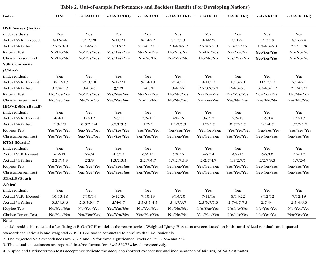
The third step of the results is on the comparison of developing and developed nations (Table 4). For developing nations, the lowest percentage failure rates are 0.3, 2, 3.7 and highest percentage failure rates are 2, 4, 7 for 1, 2.5 and 5% levels respectively. It is reported that the indices of BRICS nations have shown better performance than their developed counterparts. For developing nations (BRICS), the minimum percentage failure rate is 0.3, the maximum rate is 7. The similar values for developed nations are 1, and 8 respectively. These results exhibit strong evidence that failure rates for indices of developing nations are less than developed nations. These results imply that VaR estimates for developing nations have better results as compared to developed nations. This result of the superiority of performance (lower failure rate) by developing nations as compared to developed nations is same across all the three confidence levels and all the nine GARCH family of models (Table 2 and 3). Moreover, this paper conducts following tests for robustness of the results: 1) log likelihood ratio; 2) Ljung-Box test for serial autocorrelation; 3) ARCH-LM test for autocorrelation; 4) Nyblom stability test for variance, and 5) adjusted Pearson goodness-fit test for theory versus empirical estimates. Except for a few deviations, all the five tests of robustness, support the results of this paper (Vaz De Melo Mendes and Pereira Câmara Leal, 2005; Ali, 2013; Busch, 2005).

Discussion

6.1 Hypotheses results

As we go through the findings of this paper, we come across that I-GARCH, and e-GARCH models with both the error distributions, have given superior results. This superiority of the results has been observed across the nine indices and the three confidence levels undertaken in the study. The result implies that the first hypothesis of the paper, suitability of GARCH models to estimate VaR is dependent upon nation/index, cannot be accepted. The last section on results (section 5; step 3) and summary of best models for estimating VaR imply that the failure rate of developing nations and developed nations differ and perform better in different models. Consequently, the second hypothesis of the paper, developing and developed nations require different GARCH models to estimate VaR, can be accepted.

6.2 Policy Implication

We find that across all the ten stock indices, I-GARCH and e-GARCH models have given superior results as compared to other GARCH models. Although the results may be different from the earlier work (as explained in the next subsection 6.3), policy makers/regulators can apply the finding of this paper to re-calibrate methods to estimate VaR. This result can be justified well. Financial time series is different from other time-series due to five main features, (as discussed in subsection 4). Identified GARCH models, I-GARCH, and e-GARCH, address all the five features well. Therefore, the suggestion of re-aligning VaR estimation models in line with the findings of the paper is justified. Though, the hypothesis “suitability of the GARCH model to estimate VaR is dependent upon nation/index” cannot be accepted, we have found that the performance of developing nation is better than developed nations and have different GARCH models that perform better. This finding is relevant not only for the domestic regulatory bodies (e.g., The Securities and Exchange Board of India [SEBI] in case of India; Securities Exchange Commission [SEC] in case of USA) but also for international regulatory bodies as well (e.g., Basel Accord). Basel Accord can be modified to look for some other tool to measure market risk for developed nations. A similar adjustment is recommended for domestic regulatory bodies of developed nations to look for some tool other than VaR to measure market risks in their market.

6.3Comparison with earlier studies

Developing nations give better VaR estimates than developed nations. Literature also endorses the same. He and Wang (1995) explain that developing nations witness more noise than developed nations. As a consequence, volatility can be captured better in developing nations than in developed nations. Arago and Nieto (2005) demonstrate that, in developing nations, trading volume is more which can help in capturing volatility better than developed nations. Girad and Biswas (2007) argue that in developing nations, due to less market efficiency, volatility is more and therefore better VaR results are estimated than developed nations. However, Gaio et al., (2018) contradict with the results mentioned above and show no-difference in VaR performance between emerging and developed nations. So and Yu (2006) evince that Risk Metric is a better model at 1% confidence level. IGARCG and IGARCH-t are better at 2.5% and GARCH-t, IGARCH-t and FIGARCH-t are better at 5% confidence level in estimating VaR. However, in this paper, I-GARCH-t, I-GARCH and e-GARCH and e-GARCH models have given better results. The present study has differences in findings with So and Yu. The difference can be because both the studies are done in different nations and during different time periods. Su and Yu take data from 1995-1998 which are quite old as compared to period undertaken in this study (2010 to 2015). Su and Yo take indices of Australia, Indonesia, the UK, Hong Kong, Malaysia, South Korea, Japan, Thailand, Singapore and the USA which are considerably different from indices of the current paper. However, there are studied which support the results of the current paper (Tang and Shieh, 2006; Sethapramote, Prukumpai and Kanyamee, 2014).

McMillan and Kambouroudis (2009), Moosa and Bollen (2002) and Presecsu and Stancu (2011) show that at both the probability levels, 1% and 2.5% levels, GARCH-t (1,1) has given better results. However, at 5% level, Risk Metrics has given better results. However, in this paper, at all the probability levels, I-GARCH, and e-GARCH models (at both the Gaussian and student-t distribution for errors) have given superior results. Reason for the difference may be explained by the logic of having different indices/portfolio to test the performance of different GARCH models and having a differentperiod of the study.

6.4 Contribution of the paper

The paper has the following contributions: 1) instead of considering different GARCH model to estimate VaR, we need to only look for either I-GARCH or e-GARCH model i.e. persistent or asymmetric models to estimate VaR; 2) developing nations give better results for VaR as compared to developed nations. Therefore, to measure market risk in developed nations, another tool (other than VaR) may be considered.

7. Concluding observations

VaR is a vital market risk measurement tool which has acceptability and popularity across the world. In this study, nine types of GARCH models have been compared to estimate VaR on stock indices of developing and developed nations. Asymmetric GARCH model (estimated using e-GARCH model), and persistent models (estimated using I-GARCH) give a better estimate of VaR than other GARCH models. On the contrary, Risk Metric models and c-GARCH models perform poorly. These results are consistent for all the ten stock indices undertaken in this study, at all the three confidence levels (probability levels of 1%, 2.5%, and 5%). Stock indices of developing nations fare better than stock-indices of developed nations in estimating VaR. In other words, it can be concluded that stock-indices of developing nations are more model sensitive than developed nations for measuring VaR. These results are consistent with all the nine type of GARCH models applied in the study at all the three confidence levels. The current study has the following limitations. These limitations can be future scope of study on this topic. 1. The indices undertaken in the study are less in number. Similarly, a longer time-period could have been taken for the study. The first hypothesis; suitability of a GARCH model to estimate VaR is dependent upon nation/index; can be revisited with the larger sample size and more extendedperiod. This gap can be a future area of study. 2. A new market-risk tool can be explored for developed nations as their VaR estimates are quite less than their developing counterparts. 3. A few GARCH models like GJR GARCH and FIGARCH can be utilized in place of EGARCH and CGARCH. APARCH could also have been included in the research.

EndNote

Basel Accord is a set of guidelines given by BCBS (Basel Committee on Bank Supervisory). As of now, three sets of the guidelinehasbeen issued by BCBS (Basel 1, Basel II and Basel III). BCBS was established in 1974 to help member nations to regulate their system, especially for risk management.

References

Ahmed, S., &Zlate, A. (2014).Capital flows to emerging market economies: a brave new world?.Journal of International Money and Finance, 48, 221-248.

Aitken, M., &Siow, A. (2003).Ranking World Equity Markets on the basis of Market Efficiency and Integrity.HP Handbook of World Stock Derivative and Commodity Exchanges 2003, xlix–lv, Mondo Visione Ltd.

Ali, G. (2013). EGARCH, GJR-GARCH, TGARCH, AVGARCH, NGARCH, IGARCH and APARCH models for pathogens at marine recreational sites.Journal of Statistical and Econometric Methods, 2(3), 57-73.

Aloui, C., &Hamida, H. B. (2015). Estimation and Performance Assessment of Value-at-Risk and Expected Shortfall Based on Long-Memory GARCH-Class Models. Finance a Uver, 65 (1), 30-54.

Angelovska, J (2013). Managing market risk with VaR (Value at Risk). Journal of Contemporary Management Issues, 18(2), 81-96.

Baharumshah, A. Z., &Thanoon, M. A. M. (2006). Foreign capital flows and economic growth in East Asian countries. China economic review,17(1), 70-83.

Baillie, R. T., Chung, C. F., &Tieslau, M. A. (1996). Analysing inflation by the fractionally integrated ARFIMA-GARCH model. Journal of Applied Econometrics, 11(1), 23-40.

Bams, D., Blanchard, G., & Lehnert, T. (2017). Volatility measures and Value-at-Risk.International Journal of Forecasting,33(4), 848-863.

Beja, A. (1972). On systematic and unsystematic components of financial risk. The Journal of Finance, 27(1), 37-45.

Bekaert, G., & Wu, G. (2000). Asymmetric volatility and risk in equity markets. The Review of Financial Studies,13(1), 1-42.

Bekiros, S. D., &Georgoutsos, D. A. (2005). Estimation of Value-at-Risk by extreme value and conventional methods: a comparative evaluation of their predictive performance.Journal of International Financial Markets, Institutions and Money, 15(3), 209-228.

Berkowitz, J., &O’brien, J. (2002). How accurate are value at risk models at commercial banks?. The journal of finance, 57(3), 1093-1111.

Bollerslev, T., Chou, R. Y., & Kroner, K. F. (1992). ARCH modeling in Finance.Journal of Econometrics, 52(1/2), 5-59.

Bollerslev, T., & Mikkelsen, H. O. (1996). Modeling and pricing long memory in stock market volatility. Journal of Econometrics, 73(1), 151-184.

Boyer, B. H., Kumagai, T., & Yuan, K. (2006). How do crises spread? Evidence from accessible and inaccessible stock indices. The Journal of Finance, 61(2), 957-1003.

Brooks, C. (2014). Introductory econometrics for finance. Cambridge university press.

Brooks, C, & Persand G. (2003). Volatility forecasting for risk management. Journal of Forecasting, 22(1), 1-22.

Brooks, C., &Persand, G. (2002). Model choice and value-at-risk performance. Financial Analysts Journal, 58(5), 87-97.

Busch, T. (2005). A robust LR test for the GARCH model.Economics Letters,88(3), 358-364.

Chan, K. C., Gup, B. E., & Pan, M. S. (1997). International stock market efficiency and integration: A study of eighteen nations. Journal of Business Finance & Accounting, 24(6), 803-813.

Christofferssen, P. (1998). Evaluating Interval Forecasts. International Economic Review, 39, 841-862.

Cheng, H. F., Gutierrez, M., Mahajan, A., Shachmurove, Y., & Shahrokhi, M. (2007). A future global economy to be built by BRICs. Global Finance Journal, 18(2), 143-156.

Chong, J. (2004). Value at risk from econometric models and implied from currency options. Journal of Forecasting, 23(8), 603-620.

Degiannakis, S. (2004). Volatility forecasting: evidence from a fractional integrated asymmetric power ARCH skewed-t model.Applied Financial Economics, 14(18),1333-1342.

Degiannakis, S., Floros, C., &Dent, P. (2013). Forecasting value-at-risk and expected shortfall using fractionally integrated models of conditional volatility: International evidence. International Review of Financial Analysis, 27(1), 21-33.

Diebold, F. X., T. Schuermann, and J. D. Stroughair. (1998). Pitfalls and Opportunities in the Use of Extreme Value Theory in Risk Management.Working Paper 98–10, Wharton School, University of Pennsylvania.

Dimson, E., & Marsh, P. (1995). Capital requirements for securities firms. The Journal of Finance, 50(3), 821-851.

Ding, Z., Granger, C. W., & Engle, R. F. (1993). A long memory property of stock market returns and a new model.Journal of Empirical Finance, 1(1), 83-106.

Ding, Z., & Granger, C. W. (1996). Modeling volatility persistence of speculative returns: a new approach.Journal of Econometrics, 73(1), 85-215.

Dooley, M. P. (1988). Capital flight: a response to differences in financial risks. Staff Papers,  35(3), 422-436.

Dowd, K. (1998). Beyond value at risk: the new science of risk management. John Wiley & Sons, New York. 

Dowd, K. (2007).Measuring market risk.John Wiley & Sons.

Dungey, M., Fry, R., González-Hermosillo, B., & Martin, V. (2006). Contagion in international bond markets during the Russian and the LTCM crises. Journal of Financial Stability, 2(1), 1-27.

Enders, W. (2008). Applied econometric time series. John Wiley & Sons.

Engle, R. F., & Bollerslev, T. (1986). Modelling the persistence of conditional variances. Econometric reviews,5(1), 1-50.

Engle, R. F., & Manganelli, S. (2001). Value at risk models in finance (No. 75). ECB Working Paper, Retreived from: https://www.econstor.eu/bitstream/10419/152509/1/ecbwp0075.pdf. Accessed on 26.3.18

Fleming, J., Kirby, C., & Ostdiek, B. (2001). The economic value of volatility timing.The Journal of Finance, 56(1), 329-352.

Gaio, l. E., Pimenta Júnior, t., Lima, f. G., Passos, I. C. & Stefanelli, N. O. (2018). Value-at-risk performance in emerging and developed countries. International Journal of Managerial Finance, 14(5), 591-612.

Ghorbel, A., & Souilmi, S. (2014). Risk Measurement in Commodities Markets Using Conditional Extreme Value Theory. International Journal of Econometrics and Financial Management, 2(5), 188-205.

Girard, E., & Biswas, R. (2007). Trading volume and market volatility: Developed versus emerging stock markets. Financial Review, 42(3),429-459.

Granger, C. W., & Joyeux, R. (1980). An introduction to long-memory time series models and fractional differencing. Journal of Time Series Analysis, 1(1), 15-29.

Hamilton, J. D., & Susmel, R. (1994). Autoregressive conditional heteroskedasticity and changes in regime. Journal of Econometrics, 64(1), 307-333.

He, H., & Wang, J. (1995). Differential information and dynamic behavior of stock trading volume. The Review of Financial Studies, 8(4), 919-972.

Hoppe, R. (1999). Finance is not physics. Risk Professional, 1(7), 115-120

Holton, Glyn A (2004). Defining Risk. Financial Analysts Journal, 60(6),19-25.

Hung, J. C., Lee, M. C., & Liu, H. C. (2008). Estimation of value-at-risk for energy commodities via fat-tailed GARCH models. Energy Economics, 30(3), 1173-1191.

Hull, J. (2012). Risk Management and Financial Institutions. John Wiley & Sons, vol. 733.

Johansson, A. C., & Ljungwall, C. (2009). Spillover effects among the Greater China stock markets. World Development, 37(4), 839-851.

Karmakar, M. (2007). Asymmetric volatility and risk-return relationship in the Indian stock market.South Asia Economic Journal, 8(1), 99-116.

Karmakar, M. (2005). Modeling conditional volatility of the Indian stock markets. Vikalpa, 30(3), 21-37.

Kasman, A. (2009). Estimating Value-at-Risk for the Turkish Stock Index Futures in the Presence of Long Memory Volatility. Central Bank Review, 9(1), 1-14.

Kuester, K.; Mitinik, S.; Paolella, M. (2006). Value-at-Risk Prediction: A Comparison of Alternative Strategies. Journal of Financial Econometrics, 4, 53-89.

Kupiec, P.H. (1995). Techniques for Verifying the Accuracy of Risk Measurement Models. Journal of Derivatives,3, 73-84.

Lechner, L. A., & Ovaert, T. C. (2010). Value-at-risk: Techniques to account for leptokurtosis and asymmetric behavior in returns distributions. The Journal of Risk Finance, 11(5), 464-480.

Li, Y., & Giles, D. E. (2015). Modelling volatility spillover effects between developed stock markets and asian emerging stock markets. International Journal of Finance & Economics, 20(2), 155-177.

Lim, K. P. (2007). Ranking market efficiency for stock markets: A nonlinear perspective.Physica A: Statistical Mechanics and its Applications, 376(1-2), 445-454.

Linsmeier, T. J., & Pearson, N. D. (2000). Value at risk.Financial Analysts Journal, 56(2), 47-67.

Linsmeier, Thomas J. and Pearson, Neil, (1996). Risk Measurement: An Introduction to Value at Risk, Finance, Econ WPA. Retrieved from http://EconPapers.repec.org/RePEc:wpa:wuwpfi:9609004.

Mabrouk, S., & Aloui, C. (2010). One-day-ahead value-at-risk estimations with dual long-memory models: Evidence from the Tunisian stock market.International Journal of Financial Services Management, 4(2), 77-94.

Maghyereh, A. I. & AL-zoubi, H. A. (2006). Value-at-risk under extreme values: the relative performance in MENA emerging stock markets. International Journal of Managerial Finance,2(2), 154-172.

Maghyereh, A. I., & Awartani, B. (2012). Modeling and Forecasting Value-at-Risk in the UAE Stock Markets: The Role of Long Memory, Fat Tails and Asymmetries in Return Innovations.Review of Middle East Economics and Finance,8(1), 1-22.

McMillan, D. G., & Kambouroudis, D. (2009). Are RiskMetrics forecasts good enough? Evidence from 31 stock markets. International Review of Financial Analysis, 18(3), 117-124.    

Mensi, W. (2012). Ranking efficiency for twenty-six emerging stock markets and financial crisis: Evidence from the Shannon entropy approach. International Journal of Management Science and Engineering Management, 7(1), 53-63.

Moosa, I. A., & Bollen, B. (2002). A benchmark for measuring bias in estimated daily value at risk. International Review of Financial Analysis, 11(1), 85-100.

Nandha, M., & Hammoudeh, S. (2007). Systematic risk, and oil price and exchange rate sensitivities in Asia-Pacific stock markets. Research in International Business and Finance, 21(2), 326-341.

Nelson, D. B. (1991). Conditional heteroskedasticity in asset returns: A new approach.Econometrica: Journal of the Econometric Society,59(52), 347-370.

Nielsen, L. (2011). Classifications of countries based on their level of development: How it is done and how it could be done.IMF Working Papers, pp. 1-45.

Obi, P., Sil, S., & Choi, J. G. (2010). Value-at-risk with time varying volatility in South African equities. Journal of Global Business and Technology,6(2), 1-11.

O’Neil, J. and Poddar, T. (2008). Ten things for India to achieve its 2050 potential.Goldman Sachs Global Economic Paper No. 169, Goldman Sachs, New York, NY

Orhan, M., & Köksal, B. (2012). A comparison of GARCH models for VaR estimation.Expert Systems with Applications,39(3), 3582-3592.

Phan, K. C., & Zhou, J. (2014). Market efficiency in emerging stock markets: A case study of the Vietnamese stock market. IOSR Journal of Business and Management, 16(4), 61-73.

Philippe, J. (2001). Value at risk: the new benchmark for managing financial risk. NY: McGraw-Hill Professional.

Predescu, O. M., & Stancu, S. (2011). Value at Risk Estimation Using GARCH-Type Models. Economic Computation & Economic Cybernetics Studies & Research,45(2), 105-124.

Rastogi, S. (2010). Volatility Spillover Effect Across BRIC Nations: An Empirical Study. Paradigm, 14(1), 1-6.

Sharma, H.P., Sharma, D.K. and Alade, J.A. (2004). Value-at-risk systems and their application in integrated risk management. Journal of Academy of Business and Economics,4(1), 18-28.

Sethapramote, Y., Prukumpai, S., & Kanyamee, T. (2014). Evaluation of Value-at-Risk Estimation Using Long Memory Volatility Models: Evidence from Stock Exchange of Thailand.Retrieved from https://papers.ssrn.com/sol3/papers.cfm?abstract_id=2396531

Shao, X. D., Lian, Y. J., & Yin, L. Q. (2009). Forecasting Value-at-Risk using high frequency data: The realized range model. Global Finance Journal,20(2),128-136.

So, M. K., & Philip, L. H. Yu (2006).Empirical analysis of GARCH models in value at risk estimation. Journal of International Financial Markets, Institutions and Money,16(2),180-197.

Stiglitz, J. E. (2000). Capital market liberalization, economic growth, and instability. World Development, 28(6), 1075-1086.

Tang, T. L., & Shieh, S. J. (2006). Long memory in stock index futures markets: A value-at-risk approach. Physica A: Statistical Mechanics and its Applications, 366(1), 437-448.

Taleb, N., & Jorion, P. (1997). Against VaR.Derivatives Strategy,2(1), 21-26.

Taylor, S. (1986).Modelling  Financial time series. Wiley, New York.

Trenca, I. (2011). Advantages and Limitations of VAR Models Used in Managing Market Risk in Banks.Finante-provocarile viitorului (Finance-Challenges of the Future), 1(13), 32-43.

United Nations (2014). World Economic Situation and Prospects 2014. New York. 

Vaz De Melo Mendes, B. & Pereira Câmara Leal, R. (2005). Robust multivariate modeling in finance. International Journal of Managerial Finance,1(2), 95-106.

Vlaar, P. J. (2000). Value at risk models for Dutch bond portfolios. Journal of Banking & Finance, 24(7), 1131-1154.

Wilson, D., Kelston, A. L., & Ahmed, S. (2010). Is this the ‘BRICs decade.BRICs Monthly,10(3), 1-4.

Wilson, D., Burgi, C. and Carlson, S. (2011). A progress report on the building of the BRICs. BRICs Monthly, 11(7), 1-4.

Wilson, D., & Purushothaman, R. (2003). Dreaming With BRICs: The Path to 2050.Goldman Sachs Global Economic Paper No. 99, Goldman Sachs, New York.

Yu-dong, W. (2014). Portfolio Risk of Chinese Stock Market Measured by VaR Method. International Journal of u-and e-Service. Science and Technology,8(4), 331-338.